|
Regression
Carlos C. Rodríguez
https://omega0.xyz/omega8008/
Classical Regression
Recall the classical regression problem. Given observed data
(x1,y1),Ľ, (xn,yn) iid as a vector
(X,Y) Î Rd+1 we want to estimate f*(x) = E(Y|X=x) i.e., the regression
function of Y on X. When the vector (X,Y) is multivariate gaussian
the regression function is f*(x) = a+ L(x) with L(x) linear,
and the Ordinary (yak!) Least Squares (OLS) estimator coincides with the MLE
(Maximum Likelihood Estimator). Very often the distribution of (X,Y)
is not explicitly known beyond the n observations and the available
prior information about the meaning of these data. A typical assumption
is to think of the yj as the result of sampling the regression
function at f*(xj) with gaussian measurement error. The model is
that conditionally on x1,Ľ, xn the values of y1,Ľ,yn
are independent with Yj depending on Xj only and
Yj|Xj=xj being N(f*(xj), s2). Thus, for
j = 1,2,Ľ, n
where e1,e2,Ľ, en are iid N(0,s2).
In this way the distribution of (X,Y) is modeled semiparametrically
with (f,s) where f Î F is a function in some space of functions F
and s > 0 is a positive scalar parameter.
When F is taken as the m dimensional space F m generated by functions,
g1(x),Ľ,gm(x) estimation of the regression function reduces to
the linear optimization problem,
|
|
^
f
|
= arg |
min
f Î F m
|
|
n
ĺ
i=1
|
( yi - f(xi) )2 |
|
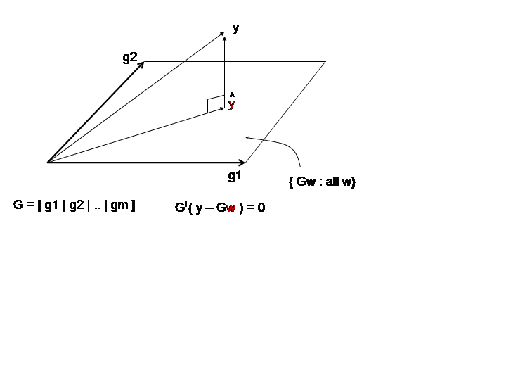
The solution is then given as the orthogonal (euclidean) projection of
the observed vector yT = (y1,y2,Ľ,yn) onto the
space generated by the columns of the matrix G Î Rm×n
with entries gij = gi(xj). In fact, the above optimization problem
can be written as,
|
|| y - |
^
y
|
||2 = |
min
w Î Rm
|
|| y - Gw ||2 |
|
 As shown by the picture, the rejection vector (i.e. y minus its projection)
must be orthogonal to the linear space generated by the columns of G,
in particular (and equivalently) to each of these columns, obtaining the
standard set of normal equations,
|
0 = GT(y - |
^
y
|
) = GT(y - G |
^
w
|
) |
|
with solution,
The more general case of Weighted Least Squares (WLS) corresponding to
the innerproduct < x,z > = xTAz generated by a symmetric positive
definite matrix A, is just,
The matrix A encodes a covariance structure for the measurement errors,
e1,Ľ,en.
Over fitting and Kernel Regression
How should F be chosen?. On the one hand, we would like F to be big so
not to constrain the form of the true regression function too much.
On the other hand, big F 's make the task of searching for the best
f Î F more difficult and more importantly without a constraint on
the explanatory capacity of F the solution will show no power of generalization.
A big enough F will always have at least one member f, able to fit all the
observations perfectly, without error, but this f provides no assurance
that f(x) is not as bad as it can possibly be for any point x not
in the training set. To be able to assure that the size of the mistake
on future data will not exceed a given value with high probability,
(i.e. to have PAC bounds) we must constrain the capacity of F somehow.
Over the years, statisticians and numerical analysts have invented all kinds
of ad-hoc devices for achieving this goal. These are known as regularization
methods. They boil down to adding a penalty term to the OLS empirical
term, often of the form W(||f||) where W is an increasing
function and F is assumed to be a space with a norm. The problem to
be solved becomes,
|
|
min
f Î F
|
|
n
ĺ
i=1
|
(yi - f(xi))2 subject to ||f|| Ł rn |
|
where the sequence of radiuses rn ® Ą as n ® Ą,
but not too quickly, (at a given rate that depends of F ) so that some
form of asymptotic stochastic convergence of the solution fn towards the
projection of the true regression function f* onto F is achieved.
Kernel Regression
Reproducing Kernel Hilbert Spaces (RKHS) provide convenient choices
for F .
- Theorem:
-
Let K be a Mercer kernel and let H K be the associated RKHS.
If
|
C((x1,y1,f(x1)),Ľ, (xn,yn,f(xn))) |
|
is any cost function that depends on f Î H K only through the
values of f(xj) at the observed xj, then the minimizer of
|
U(f) = C((x1,y1,f(x1)),Ľ, (xn,yn,f(xn))) + W(|| f ||) |
|
where W is an increasing function, is always achieved at a point
fn Î H K of the form,
|
fn(x) = |
n
ĺ
j=1
|
wj K(xj,x). |
|
Thus, when F
= H K, a big fat infinite dimensional space, the regularized
empirical cost U = C+W is minimized by solving a classic regression
problem with F n = spann{K(x1,·),Ľ, K(xn,·)}.
Proof: The proof is surprisingly simple. Every f Î H K
can be written as f = g + h where g Î F n and h Î F n^.
We show that,
with equality if and only if h=0. This follows easily from the reproducing
property of the kernel spaces. For all j Ł n,
|
f(xj) = < K(xj,·), g+h > = < K(xj,·),g > = g(xj) |
|
since h ^F n by hypothesis. Thus, C(f)=C(g). On the other hand,
since W is strictly increasing and g ^h, by the pythagorean
theorem we have,
| |
|
|
W( (||g||2 + ||h||2)1/2 ) |
| |
| |
|
| |
|
with equality if and only if h=0. Hence,
U(f) = C(g)+W(||g+h||) ł C(g)+W(||g||) = U(g). ·
Support Vector Regression
For given values a > 0, and e > 0 define the empirical cost
function ,
|
C = a |
n
ĺ
i=1
|
|yi - f(xi)|e |
|
where,
is known as the e insensitive function, and take,
With these choices, kernel regression becomes support vector regression.
The parameter e controls the sparness of the solution. The
smoothing parameter a controls the relative importance of
the empirical cost C relative to the complexity penalty W.
The derivation of the support vector regression problem follows closely
the derivation of support vector machines for classification.
We first setup a primal optimization problem for minimizing the above
e-insensitive regularized empirical cost over functions,
f(x) = < w,x > + b for the euclidean innerproduct.
Then we consider the dual problem. This turns out to be a simple
quadratic programming problem that depends on the observed data
only through the values of ( < xi,xj > ). Just as in the classification
case, we can apply the kernel trick and rip the benefits of
nonlinear kernel regression at the linear regression cost!
The Primal Problem for SV Regression
We seek the solution of,
|
minimize a |
n
ĺ
i=1
|
|yi - f(xi)|e + |
1
2
|
|
n
ĺ
i=1
|
wi2 |
|
over b,w when f(x) = < w,x > + b. This is equivalent to,
|
minimize a |
n
ĺ
i=1
|
ui + |
1
2
|
|
n
ĺ
i=1
|
wi2 |
|
over ui,wi,b
subject to: ui ł |yi-f(xi)|e for i Ł n. Each
of the last n inequalities corresponds to three inequalities,
|
ui ł 0, ui ł yi - f(xi) - e, ui ł f(xi) - yi - e |
|
Applying the standard trick of adding non negative slack variables
xi and x*i we soften the inequalities and allow
small violations. So we replace the above constrained optimization
problem with,
|
minimize a |
n
ĺ
i=1
|
ui + |
a
2
|
|
n
ĺ
i=1
|
(xi + x*i) + |
1
2
|
|
n
ĺ
i=1
|
wi2 |
|
subject to: for i Ł n,
| |
|
| |
| |
|
|
f(xi) - yi - e Ł ui + x*i |
| |
| |
|
| |
|
The objective function was chosen so that we can factorize out
a/2 and write,
|
|
a
2
|
|
n
ĺ
i=1
|
({ui+xi} + {ui+x*i}) + |
1
2
|
|
n
ĺ
i=1
|
wi2 |
|
In this way we can get rid of the ui by just replacing ui+xi by
xi and ui+x*i by x*i every where. Also, replace
a/2 by a new a to obtain the problem:
|
(Primal) minimize a |
n
ĺ
i=1
|
(xi + x*i) + |
1
2
|
|
n
ĺ
i=1
|
wi2 |
|
over, wi,b, xi, x*i subject to: for i Ł n,
The Dual Problem for SV Regression
The Lagrangian in terms of non negative Lagrange multipliers is,
| |
|
|
a |
ĺ
i
|
(xi+x*i) + |
1
2
|
|
ĺ
i
|
wi2 |
| |
| |
|
|
+ |
ĺ
i
|
li { yi - f(xi) - e- xi } |
| |
| |
|
|
+ |
ĺ
i
|
l*i { f(xi) - yi - e- x*i } |
| |
| |
|
| - |
ĺ
i
|
bi xi - |
ĺ
i
|
b*i x*i. |
| |
|
To compute the dual we need to find,
|
W(l,l*,b,b*) = |
min
w,b,x,x*
|
L |
|
The values of w,b,x,x* where the minimum is achieved must satisfy,
| |
|
| |
| |
|
| |
| |
|
| |
| |
|
|
Ű l*j + b*j = a for j Ł n. |
| |
| | |
|
Replacing these equations into L we obtain that all the terms involving xi
and x*i dissapear from L and with them, b and b*.
Therefore, W is only a function of l and l*. We get,
replacing K(xi,xj) for the innerproducts < xi,xj > (the kernel trick!) that,
| |
|
|
|
1
2
|
|
ĺ
i,j
|
(li-l*i)(lj-l*j) K(xi,xj) |
| |
| |
|
|
+ |
ĺ
i
|
(li-l*i) yi - e |
ĺ
i
|
(li+l*i) |
| |
| |
|
| - |
ĺ
i,j
|
(li-l*i)(lj-l*j) K(xi,xj) |
| |
|
The first and last terms simplify to produce,
| |
|
| |
| |
|
|
- |
1
2
|
|
ĺ
i,j
|
(li-l*i)(lj-l*j) K(xi,xj) |
| |
| |
|
| |
|
The dual problem becomes,
subject to:
where we have replaced the equalities lj+bj = a,
involving lj ł 0, bj ł 0 by the equivalent inequalities
shown above, that do not involve the bs.
As it was the case for classification, the dual problem is a simple quadratic
programming problem that can be solved with efficient algorithms that are
publicly available.
The solution from the QP solver is then used to produce the estimate,
The KKT complementarity conditions, for the slack variables are
of the type xj(lj-a) = 0 so we can write the
other complementarity conditions as follows,
are valid (and non trivial) for all
j Î J0, and j Î J*0 (resp.), where
|
J0 = { j : j Ł n, and 0 < lj < a} |
|
with J*0 defined analogously.
These, and the complementarity conditions
associated to the inequalities lj Ł a and
l*j Ł a make many lj = l*j
to be either 0 or a and producing a sparse solution. The value
for b can be obtained from any of the above complementarity conditions,
but a more accurate value is obtained by combining efforts. Replacing
the estimated values of the regression function at the training points,
|
|
^
f
|
(xj) = |
ĺ
i
|
(li-l*i) K(xi,xj) + b |
|
into the complementarity conditions, solving for b, multiplying through
by lj and l*j and adding over j Î J with
J = J0ÇJ*0 we get,
| |
|
|
|
ĺ
j Î J
|
lj{ yj - |
ĺ
i
|
(li-l*i) K(xi,xj) } |
| |
| |
|
|
ĺ
j Î J
|
l*j{ yj - |
ĺ
i
|
(li-l*i) K(xi,xj) } |
| |
|
adding the two equations, we finally obtain the estimate
|
b = |
ĺ
j Î J
|
(lj+l*j) { yj - |
ĺ
i
|
(li-l*i) K(xi,xj) } |
|
|
|
Example: SV Regression in Action
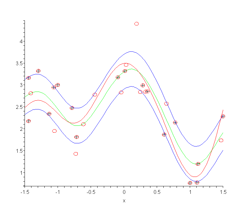
The following picture shows n=30 samples (the circles) from the true
regression line (the red curve) with gaussian error and s = 0.5.
The green curve is the estimated regression line computed using a gaussian
kernel. The blue curves show the e = 0.4 insensitive tube around
the estimate. The support vectors are marked with plus signs and a value
of a = 1.5 was used. The Maple(9.5) code is available from this site
and uses the QPsolve program in efficient matrix form from
the new Maple optimization package.

File translated from
TEX
by
TTH,
version 3.63.
On 1 Nov 2004, 15:37.
|

