Other available formats: [.PDF] [.TEX]

Learning Patterns

Carlos C. Rodríguez
https://omega0.xyz/omega8008/

Set up

We assume labeled data X Î R^d with label Y Î {0,1}. For example X=x could be the vector of pixels of a digital image of a human face and Y=1 may mean that x is the face of a woman instead of a man. The random vector (X,Y) has distribution specified by, for example, a probability measure m for X and the regression function h(x) of Y on X. We have,

P{X Î A} =

ó
õ

m(dx)

and

h(x) = P{Y=1 | X=x}

Clearly, by the sum and product rules of probability, we have

P{(X,Y) Î C} =

ó
õ

C₀

(1-h(x)) m(dx) +

ó
õ

C₁

h(x) m(dx)

where C₀ contains all the x's such that (x,0) Î C. The joint distribution of (X,Y) can be specified in other ways. Instead of picking first x according to m and then flipping a coin with probability h(x) to determine the label, we could also do it backwards.

First choose a label with (prior) probability P{Y=1} = p and then choose x with density (assuming there is one) f₀ or f₁ depending on the previously generated label y. Hence, for y Î {0,1}

P{X Î A | Y=y} =

ó
õ

f_y(x) dx

By conditioning of Y we obtain,

P{X Î A} = (1-p)

ó
õ

f₀(x) dx + p

ó
õ

f₁(x) dx =

ó
õ

m(dx)

Thus, if m has a density f(x) = m(dx)/dx it must be a mixture,

f(x) = (1-p) f₀(x) + pf₁(x)

Also, by the holy theorem,

h(x) = P{Y=1 | X=x} =

f₁(x)p

f(x)

The Bayes Classifier

A classifier is a map d: R^d ® {0,1} that assigns 0-1 labels to data vectors x Î R^d. The quality of a classifier d is measured by its risk R(d) which is simply its probability of error,

R(d) = P{d(X) ¹ Y}

The Bayes rule is the classifier d^* with smallest possible risk, so that for all d,

R(d^*) £ R(d)

We call R^*=R(d^*) the Bayes risk. It provides a measure of difficulty for the pattern recognition task at hand. It is a characteristic of the joint distribution of (X,Y).

A standard result of statistical decision theory is that the Bayes rule for the all-nothing (i.e. 0-1) loss function is the mode of the posterior distribution. Thus, d^*(x) = 1[h(x) > 1/2].

Here is an easy proof for the special case of pattern recognition. Let A(d) = {x : d(x) = 1}. Since f₁ is a density that integrates to 1, we have:

R(d) = (1-p)

ó
õ

A(d)

f₀(x) dx + p(1 -

ó
õ

A(d)

f₁(x) dx)

Which can be written as,

R(d) = p+

ó
õ

[(1-p) f₀(x) - pf₁(x)] 1_A(d)(x) dx

Notice that the rule claimed to be Bayes, assigns 1 when h(x) > 1/2 and this is equivalent to require the expression in square brackets above to be negative.

Now denote by Q(x,d) the function that is being integrated above and show that for all x Î R^d, Q(x,d^*) £ Q(x,d) (just consider each of the four cases of x in or outside A(d) and A(d^*) separately). It then follows, by the last equation above and the monotonicity of integrals, that d^* has the smallest possible probability of error and so it is the Bayes rule as claimed.

An Example

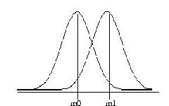
To make things concrete consider the simple case of deciding wether an observed real number x was generated by a gaussian with mean m₀ and variance 1 or a gaussian with mean m₁ and variance 1, and the two choices are considered a priori equally likely (see figure).

We want to compute the Bayes rule when the distribution of (X,Y) is characterized by p = 1/2 and f_y = N(m_y,1). For this case,

A(d^*) = { x : f₀(x) < f₁(x) } = { x :

- (x-m₀)²

- (x-m₁)²

}

and simplifies to,

A(d^*) = { x : |x-m₁| < |x-m₀| }

This shows that the best rule is to choose the distribution with mean closest to the observation x.

If we assume that m₀ < m₁ and let m=(m₀+m₁)/2 be the middle point, then the Bayes risk R^* is,

R^* =

ó
õ

¥

m

j(x-m₀) dx +

ó
õ

m

-¥

j(x-m₁) dx

By letting z=x-m₀ in the first integral, z=x-m₁ in the second and defining 2a=(m₁-m₀) we obtain a much simpler form,

R^* =

ó
õ

¥

a

j(z) dz

depending only on the separation between the two means. Here are some values,

\|m₁-m₀\|	R^*
0.1	0.480
0.5	0.401
1.0	0.309
2.0	0.159
4.0	0.023
6.0	0.001

Learning Patterns from a Teacher

If we knew the distribution of (X,Y) we could compute d^*, the Bayes rule, as shown above. Unfortunately, we rearly know the distribution of (X,Y). This creates two problems. First, we cannot directly use d^* since it depends on the parameters of the unknown distribution of (X,Y). We need to know either the sign of (h(x) - 1/2) or the sign of [(1-p)f₀(x)-pf₁(x)]. Second, we can not even evaluate the risk R(d) of any classifier d for that also depends on the unknown distribution of (X,Y).

But if we have available n independent observations (X₁,Y₁), (X₂,Y₂),¼, (X_n,Y_n) of the vector (X,Y) then we could use them to estimate the missing distribution of (X,Y) with the empirical distribution based on the observations. This could be interpreted as past data that was labeled by a reliable teacher.

Thus, we could approximate the true probability P{(X,Y) Î C} with the observed frequency given by the empirical measure n_n,

n_n(C) =

n
å
i=i

1[(X_i,Y_i) Î C]

The true risk R(d), for a given classifier d, is estimated from the observed data with the empirical risk,

(d) =

n
å
i=1

1[d(X_i) ¹ Y_i]

There is then the possibility of evaluating the quality of a d with its observed frequency of errors [^R]_n on the available data D_n=(X₁,Y₁, ¼, X_n,Y_n). But we should always keep in mind that this performance is different for different data sequences. A classifier that is built from given data D_n has as its true risk,

R_n = P{ d_n(X;D_n) ¹ Y | D_n }

Consistency

It is desirable to be able to quantify not just how good a classifier is on a fix data sequence D_n but to also know how a given classification method or rule behaves on most data sequences. In particular the notion of a consistent sequence {d_n} of classifiers is simply the requirement that,

E R_n = P{ d_n(X;D_n) ¹ Y } ® R^* as n® ¥.

A classification rule may be consistent for some distributions of (X,Y) but not for others. If however it is consistent for all of them we say that it is universally consistent. Are there any known universally consistent rules? Yes! for example the k-nearest neighbor rule (knn for short) is one of them. The knn is simply the rule that assigns to x the most common observed label among its knn's (in any metric topologically equivalent to the euclidean). Universal consistency for the knn is achieved only when k=k(n) is such that k® ¥ and k/n ®0 as n® ¥. These are the good news. The bad news: the convergence can be arbitrarily slow! Consistent rules with a given rate of convergence for all distributions of (X,Y) do not exist. This is interesting. On the one hand we know that given enough independent examples it is possible to get arbitrarily close to the performance of the Bayes rule. On the other hand it may take arbitrarily long for that to happen.

There are two ways out of this impasse. Use prior information to constraint the possible probability distributions for (X,Y) or change the target R^* by considering only a subclass C of classifiers. We take the second route first and show that there are classes C that provide universal rates of convergence to the best d_C^* for that class, i.e.,

R(d_C^*) £ R(d) for all d Î C

Empirical Risk Minimization

Let us assume that we have data D_n as above from where we can estimate the true risk of a classifier d by using the observed frequency of errors on D_n, i.e., by its empirical risk. Let d_n^* be the classifier that minimizes the empirical risk over a given class C of rules, i.e.,

(d_n^*) £

(d) for all d Î C

We would like to know what kinds of classes C allow universal empirical learning, in the sense that for all distributions of (X,Y),

R(d_n^*) ® R(d_C^*) as n ® ¥

It is intuitively clear that what's needed is some kind of constraint on the "size" (a better term would be capacity) of C. For example if C contains all possible classification functions, then no matter what the sequence D_n is, we can always find a function in this class that fits the data perfectly. However we also feel intuitively that such a rule will over fit the observed data and it will show poor performance on sequences other than the observed D_n, i.e. we expect such rule to have poor generalization power. This intuitive reasoning will be rigorously confirmed by means of the celebrated Vapnik-Chervonenkis theory.

We first notice the following simple result:

R(d_n^*) -

inf
d Î C

R(d) = R(d_n^*) -

(d_n^*) +

(d_n^*) -

inf
d Î C

R(d)

sup
d Î C

| R(d)-

(d) | +

sup
d Î C

(d) - R(d) |

The second part is trivial.

The above lemma shows that in order to achieve universal consistency on a given class, it is sufficient for the supremum appearing on the rhs of the inequalities to go to zero with probability 1, i.e., all we need to show is strong uniform convergence, over the given class, of empirical error to the true error.

File translated from T_EX by T_TH, version 3.63.
On 19 Sep 2004, 12:06.

https://omega0.xyz/omega8008/