|
Linear Classifiers
Carlos C. Rodríguez
https://omega0.xyz/omega8008/
Classification with Hyperplanes
Assume we have observed n examples of labeled data
(X1,Y1),╝,(Xn,Yn) but now let us take the labels
Y ╬ {1,-1}. This convention simplifies some of the formulas below
and it is the standard for support vector machines.
We'll be interested in classification rules of the form,
|
g(x) = sgn ( < w,x > + b ) |
|
where < , > denotes the (euclidean) inner product in Rd and w ╬ Rd and b ╬ R parametrize all the rules of this type. These
rules are called linear. The class G of linear classifiers is
about the simplest possible way of separating two kinds of objects in
Rd. A classifier in G assigns the label +1 or -1 to a data
point x ╬ Rd depending on weather we arrive to x from the plane
by going in the direction of the normal w or its oposite -w.
Recall that the set of vectors,
correspond to the hyperplane perpendicular to w that goes through every
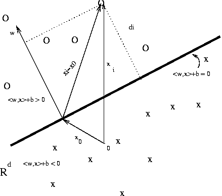
point x0 such that, < w,x0 > = -b . For example the following
picture shows such an hyperplane that perfectly separates the O's (with
label +1) from the X's (with label -1).
 The hyperplane with parameters (w,b) is the same as the hyperplane with
parameters (cw,cb) for any non-zero scalar c. To fix the scale we say
that a plane is in canonical position with respect to a set of points
X
= {x1,╝,xn } if,
|
|
min
i ú n
|
| < w,xi > + b | = 1. |
|
Clearly, the perpendicular distance from xi to the hyperplane
with parameters (w,b) is the magnitud of the projection of
(xi-x0) onto the unit normal direction w/|w|. It is given by,
|
di = |
| < w,(xi-x0) > |
|w|
|
= |
| < w,xi > + b |
|w|
|
|
|
as it can be seen from the above picture. Thus, if we assume that the
plane is in canononical position w.r.t. {xi: i ú n} then,
|
r = |
min
i ú n
|
di = |
1
|w|
|
. |
|
This minimun distance r is known as the margin between a separating
hyperplane and the points w.r.t. which that plane is in general position.
Maximum Margin Classifiers
When there is a hyperplane with
parameters (w,b) that separates the points {xi: yi = 1, i ú n}
from the points {xi: yi = -1, i ú n} then, if we take the
plane in canonical position w.r.t. X
={x1,╝,xn} we have,
|
yi( < w,xi > + b ) │ 1 for all i ú n . |
|
There could be many such planes but it is geometrically obvious that
the one farthest from the points should be prefered over all the
others. The intuition behind this is the fact that the farther the
separating boundary is from the observations the more likely it seems
for future data to end up being correctly classified by this plane. In
other words, we expect better generalization power for boundaries with
larger margin, i.e., for planes with small |w| (recall that r = 1/|w|. This intuition is confirmed by the following theorem.
- Theorem
- Consider hyperplanes through the origin in canonical position
w.r.t. X
={x1,╝,xn}. Then, the set of linear classifiers,
gw(x) = sgn < w,x > with |w| ú L has VC dimension,
where R is the radius of the smallest sphere around the origin containing
X
Before proving it notice that in fact the length of w controls the VC
dimension so that the larger the margin the larger the generalization
power as expected.
Proof:
We need to show both, V ú RdLd and V ú R2L2.
The first inequality follows from the fact that the maximum number
of spheres of radius 1/L that still fit inside a sphere of radius R
is at most vol(R)/vol(1/L) = (RL)d, where
vol(r) = Cdrd is the volume of the sphere of radius r in Rd.
More than this number of points is imposible to shatter with margin of
at least 1/L. Thus, V ú (RL)d. For the other inequality
again we show that the number of points that can be shattered with margin 1/L
is at most (RL)2. If n points can be shattered then for all possible
choices of yi ╬ {1,-1} there is an hyperplane with parameter w with
|w| ú L, in canonical position w.r.t. {x1,╝,xn} separating
+1's from -1's, i.e., satisfying,
|
yi < w,xi > │ 1 for all i=1,╝,n. |
|
But this together with Cauchy-Schwartz inequality and the fact that |w| ú L
imply,
| |
|
|
| < w, |
n
Õ
i=1
|
yixi > | ú |w| | |
n
Õ
i=1
|
yixi| |
| |
| |
|
| |
|
To bound the sum consider the case when the labels yi are Rademacher variables, i.e.
iid with P{yi=1}=1-P{yi = -1} = 1/2. From the fact that E{yiyj}=0
when i ╣ j and that yi2=1 for all i ú n, we obtain
| |
|
|
|
n
Õ
i=1
|
E{ < yixi, |
Õ
| yjxj > } |
| |
| |
|
|
|
n
Õ
i=1
|
|
ý
Ý
¯
|
Õ
j ╣ i
|
E[ < yixi,yjxj > ] + E[ < yixi,yixi > ] |
³
²
■
|
|
| |
| |
|
| |
|
If the bound is true for the expectation when Rademacher variables are used, then there
must exist yi's for which,
Squaring the initial inequality and using the above bound, we obtain
and the result follows after deviding through by n.À
File translated from
TEX
by
TTH,
version 3.63.
On 12 Oct 2004, 15:22.
|
