|
The Kernel Trick
Carlos C. Rodríguez
https://omega0.xyz/omega8008/
Why don't we do it in higher dimensions?
If SVMs were able to handle only linearly separable data, their usefulness would
be quite limited. But someone around 1992 (correct?) had a moment of
true enlightenment and realized that if instead of the euclidean inner product
< xi,xj > one fed the QP solver with a function K(xi,xj)
the boundary between the two classes would then be,
and the set of x Î Rd on that boundary becomes a curved surface embedded
in Rd when the function K(x,w) is non-linear. I don't really know
how the history went (Vladimir?), but it could have perfectly been the case that
a courageous soul just fed the QP solver with K(x,w) = exp(-|x-w|2) and
waited for the picture of the classification boundary to appear on the screen
and saw the first non linear boundary computed with just linear methods.
Then, depending on that person's mathematical training, s/he either said
aha! K(x,w) is a kernel in a reproducing kernel Hilbert space or rushed to
the library or to the guy next door to find out, and probably very soon after
that said aha!, K(x,w) is the kernel of a RKHS. After knowing about RKHS
that conclusion is inescapable but that, I believe, does not diminish the
importance of this discovery. No. Mathematicians did not know about the
kernel trick then, and most of them don't know about the kernel trick now.
Let's go back to the function K(x,w) and try to understand why, even when
it is non linear in its arguments, still makes sense as a proxy for < x,w > .
The way to think about it is to consider K(x,w) to be the inner product
not of the coordinate vectors x and w in Rd but of vectors
f(x) and f(w) in higher dimensions. The map,
is called a feature map from the data space X into the feature space H .
The feature space is assumed to be a Hilbert space of real valued functions defined
on X . The data space is often Rd but most of the interesting results
hold when X is a compact Riemannian manifold.
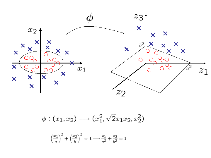
The following picture illustrates a particularly simple example where
the feature map f(x1,x2)=(x12,Ö2x1x2,x22)
maps data in R2 into R3.
 There are many ways of mapping points in R2 to points in R3
but the above has the extremely useful property of allowing the
computation of the inner products of feature vectors f(x) and
f(w) in R3 by just squaring the inner product of the
data vectors x and w in R2! (to appreciate the exclamation
point just replace 3 by 10 or by infinity!)
i.e., in this case
| |
|
| |
| |
|
|
x12w12 + 2 x1x2w1w2 + x22w22 |
| |
| |
|
| |
| |
|
| |
|
OK. But are we really entitled to just Humpty Dumpty move up to higher, even
infinite dimensions?
Sure, why not? Just remember that even the coordinate vectors x and
w are just that, coordinates, arbitrary labels, that stand as proxy
for the objects that they label, perhaps images or speech. What is
important is the inter relation of these objects as measured, for
example by the Grammian matrix of abstract inner products
( < xi,xj > ) and not the labels themselves with the euclidean dot
product. If we think of the xi as abstract labels (coordinate
free), as pointers to the objects that they represent, then we are
free to choose values for < xi,xj > representing the similarity
between xi and xj and that can be provided with a non linear
function K(x,w) producing the n2 numbers
kij=K(xi,xj) when the abstract labels xi are replaced
with the values of the observed data. In fact, the QP solver sees
the data only through the n2 numbers kij. These could,
in principle be chosen without even a kernel function and the QP solver
will deliver (w,b). The kernel function becomes useful for choosing
the classification boundary but even that could be empirically
approximated. Now, of course, arbitrary n2 numbers kij that
disregard the observed data completely will not be of much help, unless
they happen to contain cogent prior information about the problem.
So, what's the point that I am trying to make? The point is that
it is obvious that a choice of kernel function is an ad-hoc way of
sweeping under the rug prior information into the problem,
indutransductibly (!) ducking the holy Bayes Theorem. There is a kosher
path that flies under the banner of gaussian processes and RVMs
but they are not cheap. We'll look at the way of the Laplacians
(formerly a.k.a. bayesians) later but let's stick with the SVMs for now.
The question is:
What are the constraints on the function K(x,w) so that there exists
a Hilbert space H of abstract labels f(x) Î H such that
< f(xi),f(xj) > = kij ?.
The answer: It is sufficient for K(x,w) to be continuous, symmetric
and positive definite. i.e., for X either Rd or a d dimensional
compact Riemannian manifold,
satisfies,
- K(x,w) is continuous.
- K(x,w) = K(w,x). Symmetric
- K(x,w) is p.d. (positive definite). i.e., for any set
{z1,Ľ,zm} Ě X the m by m matrix
K[z] = (K(zi,zj))ij is positive definite.
Such function is said to be a Mercer kernel.
We have,
- Theorem
- If K(x,w) is a Mercer kernel then there exists a
Hilbert space H K of real valued functions defined on X and
a feature map f:X ® H K such that,
where < , > K is the innerproduct on H K.
Proof: Let L be the vector space containing all the real valued
functions f defined on X of the form,
where m is a positive integer, the aj's are real numbers and
{x1,Ľ,xm} Ě X . Define in L the inner product,
|
< |
m
ĺ
i=1
|
aiK(xi,·), |
n
ĺ
j=1
|
bjK(wj,·) > = |
m
ĺ
i=1
|
|
n
ĺ
j=1
|
aibj K(xi,wj) |
|
Since K is a Mercer kernel the above definition makes L a well
defined inner product space. The Hilbert space H K is obtained
when we add to L the limits of all the Cauchy sequences (w.r.t. the
< , > ) in L.
Notice that the inner product in HK was defined so that
|
< K(x,·), K(w, ·) > K = K(x,w). |
|
We can then take the feature map to be,
RKHS
The space HK is said to be a Reproducing
Kernel Hilbert Space (RKHS). Moreover, for all f Î H K
This follows from the reproducing property when f Î L and
by continuity for all f Î H K. It is also easy to show that the
reproducing property is equivalent to the continuity of the evaluation
functionals dx(f) = f(x).
The Mercer kernel K(x,w) naturally defines an
integral linear operator that (abusing notation a bit) we also
denote by K : H K ® H K, where,
|
(Kf)(x) = |
ó
ő
|
K(x,y) f(y) dy |
|
and since K is symmetric and positive definite, it is orthogonally
diagonalizable (just as in the finite dimensional case).
Thus, there is an ordered orthonormal basis {f1,f2,Ľ}
of eigen vectors of K, i.e., for j=1,2,Ľ
with < fi,fj > K = dij,
l1 ł l2 ł Ľ > 0 and such that,
|
K(x,w) = |
Ą
ĺ
j=1
|
ljfj(x)fj(w) |
|
from where it follows that the feature map is,
|
f(x) = |
Ą
ĺ
j=1
|
lj1/2 fj(x) fj |
|
producing,
|
K(x,w) = < f(x), f(w) > K |
|
Notice also that any continuous map f: X ® H where
H is a Hilbert space, defines K(x,w) = < f(x),f(w) > which is
a Mercer Kernel.
File translated from
TEX
by
TTH,
version 3.63.
On 25 Oct 2004, 14:37.
|
