A basic problem of statistical inference is to estimate the probability distribution that generated the observed data. In order to allow the data to speak by themselves, it is desirable to solve this problem with a minimum of a priori assumptions on the class of possible solutions. For this reason, the last thirty years have been burgeoning with interest in nonparametric estimation. The main positive results are almost exclusively from non-Bayesian quarters, but due to recent advances in Monte Carlo methods and computer hardware, Bayesian nonparametric estimators are now becoming more competitive.
This paper aims to extend the idea in [1] to a new general Bayesian approach to nonparametric density estimation. As an illustration one of the techniques is applied to compute the estimator in . In particular it is shown how to approximate the bayes estimator (for Jeffreys' prior and quadratic loss) for the bandwidth parameter of a kernel using a version of the metropolis algorithm. The computer experiments with simulated data clearly show that the bayes estimator with Jeffreys' prior outperforms the standard estimator produced by plain Cross-validation.
Any non-Bayesian nonparametric density estimator can be turned into a Bayesian one by the following three steps:
The summing over paths method, springs from the simple idea of interchanging sums and products in the expression for the cross-validated kernel likelihood (see [1]). Without further reference to its humble origins, let us postulate the following sequence of functions,
| (1) |
Notice that by flipping the sum and the product we get
| (2) |
| (3) |
The Fn's can be used as a universal method for attaching a class of exchangeable one parameter models to any set of observations. The positive scalar parameter h is the only free parameter, and different models are obtained by changing the kernel function K.
These empirical parametric models are invariant under relabeling of the observations (i.e. they are exchangeable) but they do not model the observations as independent variables. Rather, these models introduce a pattern of correlations for which there is a priori no justification. This suggest that there might be improvements in performance if the sum is restricted to special subsets of the set of all nn+1 paths. Three of these modifications are mentioned in the following section.
Notice also that the ability of the Fn to adapt comes at the expense of regularity. These models are always non-regular. If the kernel has unbounded support then Fn integrates to infinity but the conditional distribution of x0 given x1,Ľ,xn and h is proper. When the kernel has compact support the Fn are proper but still non-regular since their support now depends on h.
The above recipe would have been a capricious combination of symbols if it not were for the fact that, under mild regularity conditions, these models adapt to the form of the true likelihood as n increases.
As a function of x0 = x, the Fn have the following asymptotic property,
Theorem 1
If x1,x2,Ľ,xn are iid observations from an unknown pdf f which is
continuous a.s. and h = hn is taken as a function of n such that, hn® 0 and nhn® Ą as n® Ą, then,
Fn
ó
ő
Fndx0
= f-0,n(x)+o(1) = f(x)+o(1). (4)
Proof (sketch only)
Just flip the sum and the product to get again,
| (5) |
It is worth noticing that the above theorem is only one of a large number of results that are readily available from the thirty years of literature on density estimation. In fact under appropriate regularity conditions the convergence can be strengthen to be pointwise a.s., uniformly a.s., or globally a.s. in L1, or L2.
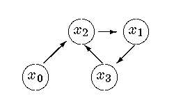
Each of the nn+1 paths (i0,Ľ,in) can be represented by a graph with nodes x0,Ľ,xn and edges from xj to xk if and only if ij = k. Here are some graphs for paths with n = 3. For example, the path (2,3,1,2) is given a probability proportional to
| (6) |

The path (1,2,3,0) is the single ordered loop of size four (a 4-loop), (3,0,1,2) is the same loop backwards (also a 4-loop), (2,3,0,1) are two disconnected loops (a 2-2-loop) and (1,0,0,0) is connected and contains a loop of size two with x0 and x1 in it (a 1-1-2-loop). Draw the pictures!
The classification of paths in terms of number and size of loops appears naturally when trying to understand how Fn distributes probability mass among the different paths. To be able to provide simple explicit formulas let us take K in the definition of Fn to be the standard gaussian density, i.e. from now on we take,
| (7) |
| ||||||||||||||||||||||||
| (10) |
Theorem 2
ó
ő
m1-m2-Ľ-mk-loop
=
ć
č
ó
ő
m1-loop
ö
ř
ć
č
ó
ő
m2-loop
ö
ř
Ľ
ć
č
ó
ő
mk-loop
ö
ř
(11)
ó
ő
m-loop
= (2p)-1/2
h-1
Öm
L (12)
Proof
Equation (11) follows from Fubini's theorem. To get (
12) use Fubini's theorem and apply (10) each time to
obtain,
| ||||||||||||||||||||||||||||||||||||||||||
|
| (13) |
Preliminary simulation experiments seem to indicate that only maximally disconnected paths are not enough and that all the loops are too many. The QM method has all the maximally disconnected paths but not all the loops (e.g. with n = 5 the 3-3-loops can not be reached by squaring the sum of 2-2-2-loops) so it looks like the most promising among the three. What is more interesting about the QM method is the possibility of using kernels that can go negative or even complex valued. More research is needed since very little is known about the performance of these estimators.
We show in this section how to approximate the predictive distribution and the bayes rule for the smoothness parameter by using Markov Chain Monte Carlo techniques.
Apply bayes' theorem to (1) to obtain the posterior distribution of h,
| (14) |
| (15) |
| (16) |
| (17) |
| (18) |
| (19) |
| (20) |
To approximate equation (17) we use the fact that the ratio of
the two sums is the expected value of a random variable that takes the value
s(i) on the path i which is generated with
probability proportional to a(i). The following version
of the Metropolis algorithm produces a sequence of averages that converge to
the expected value,
Algorithm
0) Start from somewhere
i ¬ (1,2,Ľ,n,0)
s2 ¬ ĺj = 0n (xj - xij)2
a¬ (s2)-(n+d)/2
N ¬ 0, sum ¬ 0, ave ¬ 0
1) Sweep along the components of i
for k from 0 to n do
{
i˘k ¬ Uniform on {0,Ľ,n}\{k,ik}
Dk ¬ (xi˘k-xik) (xi˘k+xik-2xk)
s2˘ ¬ s2 + Dk
a˘ ¬ (s2˘)-(n+d)/2
R ¬ a˘/a
if R > 1 or Unif[0,1] < R then {ik ¬ i˘k,s2¬ s2˘, a¬ a˘}
}
2) Update the estimate for the average,
sum ¬ sum +[Ös2]
N¬ N+1
ave ¬ sum/N
goto 1)
To sample from the predictive distribution, f(x|x1,x2,Ľ,xn) we use Gibbs to sample from the joint distribution, f(x,h|x1,x2,Ľ,xn). Hence, we only need to know how to sample from the two conditionals, a) f(x|h,x1,x2,Ľ,xn) and b) p(h|x,x1,x2,Ľ,xn). To sample from a) we use the fact that this is (almost) the classical kernel so all we need is to generate from an equiprobable mixture of gaussians. To get samples from b) just replace the gaussian kernel into the numerator of equation (14) to obtain, for p(h) µ h-d,
| (21) |
| (22) |
| (23) |
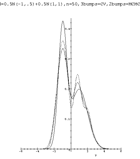
I have coded (essentially) the algorithm described in the previous section in MAPLE and tested it dozens of times on simulated data for computing a global value for the smoothness parameter h. All the experiments were carried out with d = 1 i.e. with p(h) = h-1 on mixtures of gaussians. The experiments clearly indicate that the global value of h provided by the MCMC algorithm produce a kernel estimator that is either identical to plain likelihood cross-validation or clearly superior to it depending on the experiment. A typical run is presented in figure [2 ] where the true density and the two estimators from 50 iid observations are shown. The MAPLE package used in the experiments is available at https://omega0.xyz/omega8008/npde.mpl.

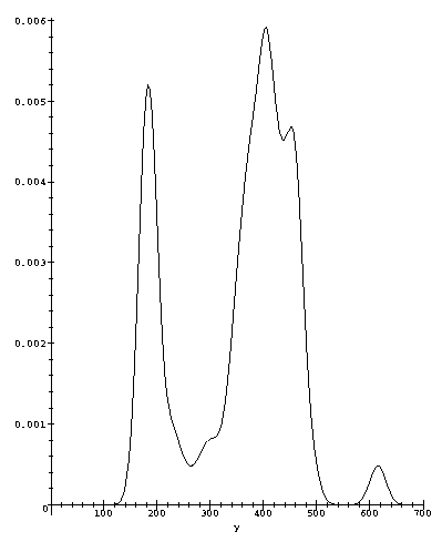
For comparison with other density estimators in the literature we show in figure [3] the estimate for the complete set of 109 observations of the Old Faithful geyser data. These data are the 107 observations in [2] plus the two outliers 610 and 620. This is a standard gaussian kernel with the global value of h = 14.217 chosen by the MCMC algorithm.

There is nothing special about dimension one. Only minor cosmetic changes (of the kind: replace h to hd in some formulas) are needed to include the multivariate case, i.e. the case when the xj's are d-dimensional vectors instead of real variables.
Very little is known about these estimators beyond of what it is presented in this paper, In particular nothing is known about rates of convergence. There are many avenues to explore with theory and with simulations but clearly the most interesting and promissing open questions are those related to the performance of the QM method above.