Partial Derivatives

We want to apply the concept of derivative to a function of several variables. Suppose f is a function of x and y. If we let only x vary while keeping y=b fixed at the value b we have a function of a single variable:
g(x) = f(x,b) If the derivative of g exists at x=a we call it the partial derivative of f with respect to x at (a,b) and we write it by either fx(a,b) or D1f(a,b). We have

> #


                    df                  f(a + t, b) - f(a, b)
                   ---(a,b)  = Limit    ---------------------
                    dx         t -> 0           t

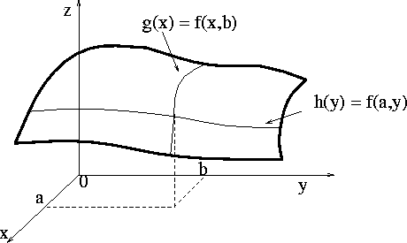
The partial derivative of f w.r.t. x can be seen as the rate of change of the value of the function with respect to a change in x when y is kept constant. If we visualize the graph of the function z = f(x,y) as a surface above the xy plane then the partial derivative of f w.r. to x at (a,b) is the slope of the line of intersection of the surface with the plane y=b at the point (a,b,f(a,b)). The following picture shows a surface z=f(x,y) and the graphs of the two curves z=g(x)=f(x,b) and z=h(y)=f(a,y),

The slope of the tangent line to z=g(x) at x=a is the partial derivative of f w.r.t. x at (a,b) and the slope of the tangent line to z=h(y) at y=b is the partial derivative of f w.r.t. y at (a,b). To compute partial derivatives all you have to do is to compute regular derivatives assuming all (but the variable you are computing the derivative w.r.t.) the other variables as if they were constants.

The following picture shows how the plane x=a cuts the surface z=f(x,y) in full animation,

cutting z=f(x,y) with x=a

Here are several examples with maple:

> f1 := (x,y) -> 4*x^2*y-sin(3*y);


                                          2
                        f1 := (x,y) -> 4 x  y - sin(3 y)

> Diff('f1(x,y)',x) = diff(f1(x,y),x);


                               d
                             ---- f1(x, y) = 8 x y
                              dx

> Diff('f1(x,y)',y) = diff(f1(x,y),y);


                         d                2
                       ---- f1(x, y) = 4 x  - 3 cos(3 y)
                        dy

Higher order partials are defined by just taking the derivatives of derivatives.....Look at this examples

Link to the commands in this file

Carlos Rodriguez <carlos@math.albany.edu>

Last modified: Thu Oct 10 17:20:54 EDT 1996