| There are several ways to compute partial derivatives of a function of sevaral variables using Maple. First it depends on how the expression for the function is entered to Maple. We can enter the function as an expression in x,y,z etc... like: |
> f := 3*z^2*cos(x*z)+x^2/(y^2+sin(y)^2*z);
                                                  2
                              2                  x
                      f := 3 z  cos(x z) + --------------
                                            2         2
                                           y  + sin(y)  z
| Partial derivatives can now be computed with "diff". The partial derivative of f with respect to x at an arbitrary point (x,y,z) is given by: |
> Dfx := Diff(f,x) = diff(f,x);
 Dfx :=

          /                       2      \
       d  |   2                  x       |        3                     x
     ---- |3 z  cos(x z) + --------------| = - 3 z  sin(x z) + 2 --------------
      dx  |                 2         2  |                        2         2
          \                y  + sin(y)  z/                       y  + sin(y)  z
| If there is a need for evaluating the partials at different values of x,y,z then it is often more convenient to "unapply" the previous expression and then use the function to evaluate. The alternative would be to use "subs" for substitutions. |
> fx := unapply(op(Dfx)[2],x,y,z);
                                    3                     x
              fx := (x,y,z) -> - 3 z  sin(x z) + 2 --------------
                                                    2         2
                                                   y  + sin(y)  z
fx(1,1,0) = 2
fx(1,1,0) = 2
| Mixed partials can be computed with the help of the "$" sequence operator, |
> Diff('f',x,y$2) = diff(f,x,y$2);
    Diff(f, x, y, y) =

                                     2                    2             2
          x (2 y + 2 sin(y) z cos(y))      x (2 + 2 cos(y)  z - 2 sin(y)  z)
        4 ---------------------------- - 2 ---------------------------------
                  2         2   3                    2         2   2
                (y  + sin(y)  z)                   (y  + sin(y)  z)
The previous expression is the third order partial derivative of f with respect to x,y and y. Maple assumes that the mixed partials are continuous
so it doesn't care about the order. Watch out.
ExercisesProblem1:Compute the partial derivative of f1 w.r. to x at the points (1,2) and (2,1). Interpret these numbers as slopes and illustrate with sketches. |
> f1 := (x,y) -> 16-4*x^2-y^2;
                                                2    2
                         f1 := (x,y) -> 16 - 4 x  - y
Solution1:To compute the partial derivative we can use the differential operator D |
> g := unapply(f1(x,2),x); fx := D(g);
                                                2
                              g := x -> 12 - 4 x

                                fx := x -> - 8 x
| The partial evaluated at (1,2) is then, |
> `fx(1)` = fx(1);
fx(1) = -8
| The partial evaluated at (2,1) is given by, |
> gx := subs({x=2,y=1},diff(f1(x,y),x));
gx := -16
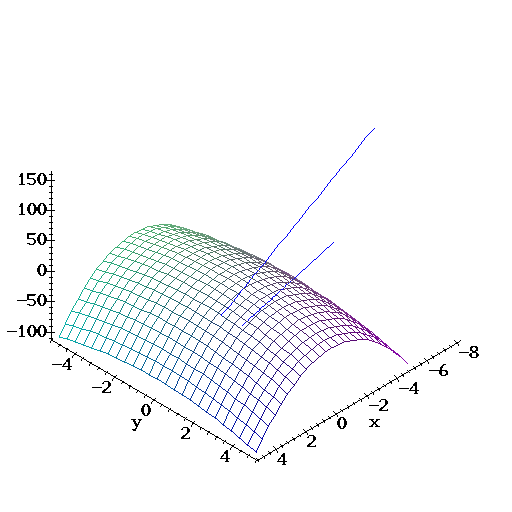
| This means that at the point (1,2,8) the tangent plane to the surface z = f1(x,y) has a slope of -8 in the x-direction. At the point (2,1,-1) it has slope -16. To plot the surface and the two tangent lines we create the pictures one at a time, and then display them with display3d. |
> S := plot3d(f1(x,y),x=-5..5,y=-5..5,axes=framed):
> with(plots):
> L1 := spacecurve(evalm([1,2,8]+t*[1,0,-8]),t=-5..1,color=yellow):
> L2 := spacecurve(evalm([2,1,-1]+t*[1,0,-16]),t=-10..1/16,color=yellow):
> display3d({S,L1,L2},axes=framed);

| Do you see why the definitions of L1 and L2 are correct? Do it! |
Problem2:Verify that the function: |
> u := (x,t) -> exp(-a^2*k^2*t)*sin(k*x);
                                          2  2
                     u := (x,t) -> exp(- a  k  t) sin(k x)
| is a solution of the so called heat conduction equation: |
> #
                             d       2
                           ---- u = a  Diff(u, x, x)
                            dt
Solution2:All we need to do is to let maple check, |
> ut := diff(u(x,t),t);
                              2  2        2  2
                     ut := - a  k  exp(- a  k  t) sin(k x)
                               2  2        2  2
                     Rhs := - a  k  exp(- a  k  t) sin(k x)
| So YES! it is a solution since, |
> ut - Rhs;
0