| Let f be the following function of the real variable x, |
> f := x -> (x+2) / (3+(x^2+1)^3);
                                          x + 2
                            f := x -> -------------
                                            2     3
                                      3 + (x  + 1)
> D(f);
                                                    2     2
                              1           (x + 2) (x  + 1)  x
                   x -> ------------- - 6 -------------------
                              2     3              2     3 2
                        3 + (x  + 1)        (3 + (x  + 1) )
| Notice that D(f) returns the derivative of f as a function. Think of D(f) as the usual f' (i.e. f-prime the derivative of f) |
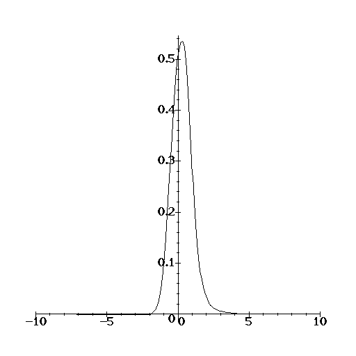
> plot(f);

| The first time let Maple adjust the x and y ranges. |
> f(0);
1/2
| Do you see that the global max of f is at an x a bit bigger than 0 ? |
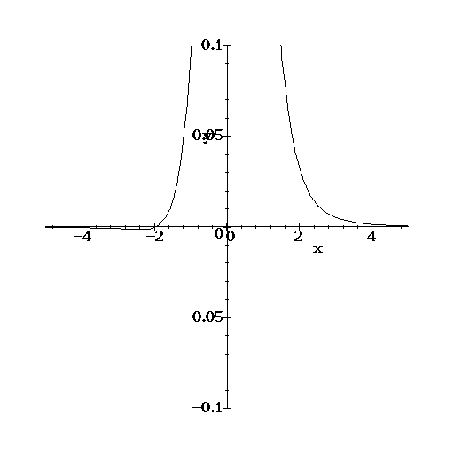
> plot(f(x), x=-5..5, y=-0.1..0.1);

                             6      4      2       5       3
                    - 4 + 5 x  + 9 x  + 3 x  + 12 x  + 24 x  + 12 x
             d := - -----------------------------------------------
                                      6      4      2 2
                                (4 + x  + 3 x  + 3 x )
> fsolve(numer(d));
-2.485165927, .2700964050
| Let's grab this list of two numbers for later use. |
> s := ";
s := -2.485165927, .2700964050
| A quick check... |
> D(f)(s[2]);
                                         -9
                                    .1*10
|
VERY close to 0 as it should. Why isn't exactly zero? Now the inflection points... We use now the command "diff" instead of "D".... See the difference? |
> diff(d,x);
      5       3             4       2
  30 x  + 36 x  + 6 x + 60 x  + 72 x  + 12
- ----------------------------------------
                 6      4      2 2
           (4 + x  + 3 x  + 3 x )

                   6      4      2       5       3             5       3
         (- 4 + 5 x  + 9 x  + 3 x  + 12 x  + 24 x  + 12 x) (6 x  + 12 x  + 6 x)
     + 2 ----------------------------------------------------------------------
                                       6      4      2 3
                                 (4 + x  + 3 x  + 3 x )
| Use 'simplify' to combine the two fractions into a single one. |
> simplify(");
            5      11       9       7       3              4       10       8
   6 (- 19 x  + 5 x   + 17 x  + 18 x  - 37 x  - 12 x + 14 x  + 14 x   + 54 x

              6       2        /       6      4      2 3
        + 76 x  - 30 x  - 8)  /  (4 + x  + 3 x  + 3 x )
                             /
> fsolve(numer("));
-2.964270928, -.5472819999, .8702050673
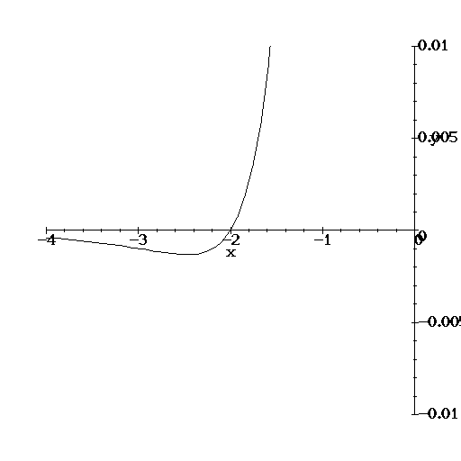
| So these are the x locations of the three inflection points. Had we used 'solve' instead of 'fsolve' we would have obtained the exact values but usually at the expense of complicated expresions. We can now adjust the x and y ranges to see what's going on to the left of 0. |
> plot(f(x), x=-4..0, y=-0.01..0.01);

| Do you see the inflection pt. around -3 ? Also, do you see the global min of f.. at around s[1] = -2.5 ? |