|
|
Heights of the Blocks
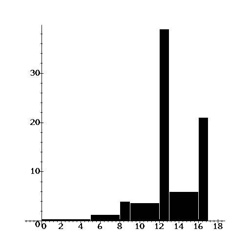
| First lets compute the heights of the blocks on top of each of the intevals. Remember that the AREA of the block matches the % of entries in the list in that interval. Thus, |
> Percent := [2,4,4,11,39,18,21];
Percent := [2, 4, 4, 11, 39, 18, 21]
> width := [5-0,8-5,9-8,12-9,13-12,16-13,17-16];
width := [5, 3, 1, 3, 1, 3, 1]
> Mid := [2.5,6.5,8.5,10.5,12.5,14.5,16.5];
Mid := [2.5, 6.5, 8.5, 10.5, 12.5, 14.5, 16.5]
| The previous list are the mid points of each of the intervals. To compute the heights just devide the Percent by the width for each interval. Here is the calculation for the 4th interval (9,12]: |
> Height4 := Percent[4]/width[4];
Height4 := 11/3
| or approximately |
> H4 := evalf(11/3,2);
H4 := 3.7
| So here is the calculation for all the intervals... |
> H := [seq(evalf(Percent[k]/width[k],2),k=1..7)];
H := [.40, 1.3, 4., 3.7, 39., 6., 21.]
| Let us now draw the histogram, |
> with(stats): with(stats[statplots]):
> data1 := [Weight(0..5,2), Weight(5..8,4), Weight(8..9,4), Weight(9..12,11),
> Weight(12..13,39), Weight(13..16,18), Weight(16..17,21)];
     data1 := [Weight(0 .. 5, 2), Weight(5 .. 8, 4), Weight(8 .. 9, 4),

         Weight(9 .. 12, 11), Weight(12 .. 13, 39), Weight(13 .. 16, 18),

         Weight(16 .. 17, 21)]
> histogram(data1);

|
|
The AVE
| Let us now compute the average from the distribution table. First notice that the distribution table has only imcomplete information about the list since the data has been bined into the intervals. In fact we do not even know the number of entries in the original list of numbers! But it doesn't matter... we can still compute a good approximation for the average of the original list just with the information provided by the table. Think about it this way: > If there were 100 entries in the list (by the way there were probably several million in the list used to build the table for this problem...) then 2 of those 100 will be numbers in the first interval i.e. 2 people out of the 100 will have less than five years of schooling, 4 people will have between 5 and 8 years of schooling ... etc... Since we do not know where within the interval those people actually are we should guess they are all at the center (the mid point of each interval). In this way we can reconstruct an approximation of the original list from which we can compute everything, Average, SD, Median etc... Hence, |
> Average := Sum(Percent[j]*Mid[j],j=1..7)/100;
                                    /  7                    \
                                    |-----                  |
                                    | \                     |
                   Average := 1/100 |  )   Percent[j] Mid[j]|
                                    | /                     |
                                    |-----                  |
                                    \j = 1                  /
| which evaluates to, |
> Average := sum(Percent[j]*Mid[j],j=1..7)/100;
Average := 12.75500000
|
|
The SD
| To compute the SD we use the approximate list as above and the formula for the SD, |
> SD := sqrt( Sum(Percent[i]*(Mid[i]-Average)^2,i=1..7)/100);
                       /  7                                     \1/2
                       |-----                                   |
                       | \                                     2|
            SD := 1/10 |  )   Percent[i] (Mid[i] - 12.75500000) |
                       | /                                      |
                       |-----                                   |
                       \i = 1                                   /
| which evaluates to: |
> SD := sqrt( sum(Percent[i]*(Mid[i]-Average)^2,i=1..7)/100);
SD := 2.910425184
|
|
The Median
| Recall that the Median is the entry in a list of numbers such that 50% of the entries in the list are smaller than it and the other 50% above it. So... the median is clearly between 12 and 13. More exactly... |