Correlation and Regression Examples

Problem:

In a (hypothetical) study on population growth, data on the percentage of kids of different ages is collected for 10 cities.

	Age	% of Population
      __________________________
	1		4
	1		5
	1		7
	1		3
	2		3
	2		3
	2		1
	3		1
	3		1
	4		1

Compute the 5 number summary for these data
Show the scatter plot.
Find the least squares regression line of % on Age
Plot the cloud of points, the SD line and the regression line of % on Age.
Compute the R.M.S. error for the regression of % on Age.
A kid who is 3.5 years of age is expected to belong to a city containing what % of kids her age?
What % of the kids who are 3.5 years of age are expected to be in cities with more that one percent of kids of their age?

SOLUTIONS:

First let's enter the data to the calculator.

> with(stats): age := [1,1,1,1,2,2,2,3,3,4];

                     age := [1, 1, 1, 1, 2, 2, 2, 3, 3, 4]

> ppop := [4,5,7,3,3,3,1,1,1,1];

                    ppop := [4, 5, 7, 3, 3, 3, 1, 1, 1, 1]

> ave := dat -> stats[describe,mean](dat):
> sd := dat -> stats[describe,standarddeviation](dat):
> r := (x,y) -> stats[describe,linearcorrelation](x,y):
> aveAge := ave(age); sdAge := sd(age); avepp:= ave(ppop);sdpp:=sd(ppop);

                                  aveAge := 2

                                  sdAge := 1


                                  avepp := 2.9


                              sdpp := 1.92

> rAp := r(age,ppop);

    
                              rAp := - 0.78

> scatter:=(x,y) -> stats[statplots,scatterplot](x,y):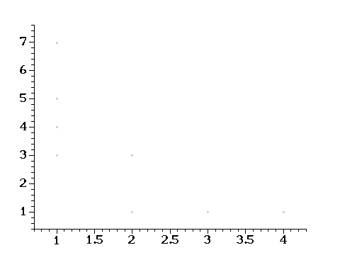
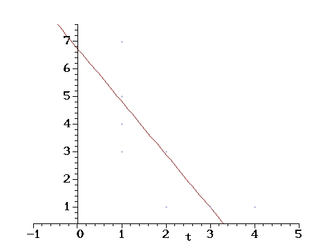
> scatter(age,ppop);
picture a picture here

Scatter plot with the SD line

> sdline := t -> 2.9 - 1.92*(t-2):
> l1 := plot(sdline(t),t= -1..5): scatt := scatter(age,ppop):
> with(plots):
> display({l1,scatt});

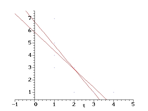
Both the SD and the Regression line

Recall that the regression line is the line that minimizes the sum of the squeares of the residuals and it is also known as the line of least squares.

> rl := plot(2.9 - 0.78*1.92*(t-2),t=-1..5):
> display({l1,rl,scatt});

The R.M.S. for % on Age

> RMS := sqrt(1 - 'r'^2)*SDy;

                                         2 1/2
                            RMS := (1 - r )    SDy

For our data this is:

> RMS := sqrt(1. - 0.78^2)*1.92;

                              RMS := 1.2

When age = 3.5 the regression line predicts:

To get y from x using the regression line of y on x do:

transform x to standard units
multiply by r to obtain y in standard units
transform y to its original units

> x_in_sus := (3.5 - ave(age))/sd(age);

                                x_in_sus := 1.5

> y_in_sus := x_in_sus * r(age,ppop);

                        y_in_sus := -1.2

> y_predicted := ave(ppop) + y_in_sus * sd(ppop);

                           y_predicted := 0.65

What proportion of the kids, who are 3.5 years of age, belong to cities with more than 1% of kids their age?

Here we are looking only at 3.5 year olds. We use the fact that the list of y values (in this case pop. %) with a fix value of x (in this case age=3.5) follows the normal curve with an average given by the regression line (y when x=3.5) and an SD estimated by the R.M.S. error for the regression of y on x. Thus the question is: What proportion of the entries of a list that follows the normal curve with ave = 0.65 and SD= 1.2 is expected to be greater than 1?

answer:

transform the interval to standard units
look up the percent of area under the normal curve

> a_in_sus := (1 - 0.65)/1.2;

                            a_in_sus := 0.29

The area under the normal curve to the right of 0.29 is computed from the area given on the table for z = 0.29


  z    Height  Area     z    Height  Area     z    Height  Area 
___________________    __________________    ___________________
 0.00  39.89   0.00    1.50  12.95  86.64    3.00  0.443  99.730
 0.05  39.84   3.99    1.55  12.00  87.89    3.05  0.381  99.771
 0.10  39.70   7.97    1.60  11.09  89.04    3.10  0.327  99.806
 0.15  39.45  11.92    1.65  10.23  90.11    3.15  0.279  99.837
 0.20  39.10  15.85    1.70   9.40  91.09    3.20  0.238  99.863

 0.25  38.67  19.74    1.75   8.63  91.99    3.25  0.203  99.885
 0.30  38.14  23.58    1.80   7.90  92.81    3.30  0.172  99.903
 0.35  37.52  27.37    1.85   7.21  93.57    3.35  0.146  99.919
 0.40  36.83  31.08    1.90   6.56  94.26    3.40  0.123  99.933
 0.45  36.05  34.73    1.95   5.96  94.88    3.45  0.104  99.944

Hence, the area between -0.29 and +0.29 is about 23.5% so the area outside this interval (both tails) is about 76.5% and the right tail is just half of this i.e.

> Answer := (100 - 23.5)/2;

                             Answer := 38 %

Link to the commands in this file

Carlos Rodriguez <carlos@math.albany.edu>

Last modified: Tue Mar 16 13:27:06 EST 1999