The Normal Curve can be used as an ideal histogramThe Equation and picture of the Normal (or Gaussian) Curve are: |
> y := 100*exp(-x^2/2)/sqrt(2*Pi);
                                             2   1/2
                                  exp(- 1/2 x ) 2
                          y := 50 ------------------
                                          1/2
                                        Pi
> plot(y,x=-4..4,labels=["Standard Units",""]);
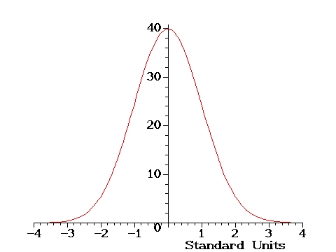
The area under the normal curve between -1 and 1 is about 68%The area under the normal curve between -2 and 2 is about 95%The area under the normal curve between -3 and 3 is about 99%Many histograms for data are similar to the normal curve provided that they are drawn to the same scale of STANDARD UNITS.STANDARD UNITS say how many SDs above or below the AVE a value is |
> Example:
| The average score in last year's MAT108 final exam was 53 points, with an SD of 18 points. Aaron scored 48 pts. and Cecilia 74 on the final last year. What were there scores in standard units? |
> Answer:
| To convert from the original units to standard units just find out how many SDs above or below the AVE that number is. Thus, |
> Aaron_SUs := (48 - 53)/18.; Cecilia_SUs := (74-53)/18.;
                           Aaron_SUs := -.2777777778

                          Cecilia_SUs := 1.166666667
> Question: | What score corresponds to -2.5 standard units? |
> Answer:
| To convert from SUs to original units just add to the AVE the given SUs times the SD. |
> Score := 53*pts + (-2.5)*18*pts;
Score := 8.0 pts
| i.e. 8 pts is the score which is 2.5 SDs below the AVE. |
The following data are the scores in another Statistics Exam. |
> read `scores.mpl`;
scores := [68, 74, 55, 92, 71, 73, 45, 59, 46, 42, 54, 71, 71, 52, 72, 85, 42,

    27, 16, 90, 62, 83, 32, 81, 79, 56, 100, 92, 90, 46, 79, 51, 59, 29, 89,

    63, 80, 52, 72, 51, 38, 33, 46, 52, 30, 64, 64, 59, 88, 58, 62, 46, 16, 75,

    81, 24, 66, 35, 70, 22, 41, 96, 40, 71, 51, 43, 94, 79, 52, 92, 46, 38, 53,

    29, 82, 72, 65, 73, 84, 77, 36, 93, 82, 83, 42, 53, 69, 51, 79, 45, 51, 53,

    86, 89, 52, 63, 78, 70, 0, 37, 35, 34, 67, 57, 92, 87, 69, 62, 36, 51, 69,

    31, 61, 100, 52, 71, 83, 74, 36, 80, 34, 58, 59, 85, 100]
> with(statplots): 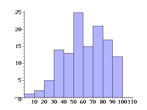
To compare the above histogram against the normal curve you must transform the scores to STANDARD UNITS. |
> read `ToSus.mpl`;
ToSUs := proc(alist, ave, sd)
local i, newList;
    for i to nops(alist) do newList[i] := (alist[i] - ave)/sd od;
    RETURN(newList)
end
> with(stats): with(describe): AVE := 61.2> SD := evalf(sqrt(variance(scores)),3);
SD := 21.1
Let's transform the scores into SUs |
> scrs_in_SUs := evalf(ToSUs(scores,AVE,SD),2);
scrs_in_SUs := [.33, .62, -.29, 1.5, .48, .57, -.76, -.095, -.71, -.90, -.33,

    .48, .48, -.43, .52, 1.1, -.90, -1.6, -2.1, 1.4, .048, 1.0, -1.4, .95, .86,

    -.24, 1.9, 1.5, 1.4, -.71, .86, -.48, -.095, -1.5, 1.3, .095, .90, -.43,

    .52, -.48, -1.1, -1.3, -.71, -.43, -1.5, .14, .14, -.095, 1.3, -.14, .048,

    -.71, -2.1, .67, .95, -1.8, .24, -1.2, .43, -1.9, -.95, 1.7, -1.0, .48,

    -.48, -.86, 1.6, .86, -.43, 1.5, -.71, -1.1, -.38, -1.5, 1.0, .52, .19,

    .57, 1.1, .76, -1.2, 1.5, 1.0, 1.0, -.90, -.38, .38, -.48, .86, -.76, -.48,

    -.38, 1.2, 1.3, -.43, .095, .81, .43, -2.9, -1.1, -1.2, -1.3, .29, -.19,

    1.5, 1.2, .38, .048, -1.2, -.48, .38, -1.4, 0, 1.9, -.43, .48, 1.0, .62,

    -1.2, .90, -1.3, -.14, -.095, 1.1, 1.9]
> with(statplots): with(plots): 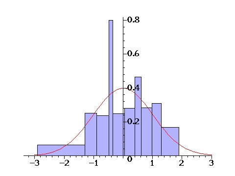
Now Areas under the histogram can be approximated by Areas under the Normal Curve.Small areas don't match up very well but this improves for larger areas.For Example: about 16% of the scores should be less than -1 SUs = 40.1 pts.By looking at the data we see that |
> sort(scores);
[0, 16, 16, 22, 24, 27, 29, 29, 30, 31, 32, 33, 34, 34, 35, 35, 36, 36, 36, 37,

    38, 38, 40, 41 ... 100]
21 out of the 125 scores, 16.8%, were actually below 40. |