Lecture VIII
An Introduction to Markov Chain Monte Carlo

Lecture VIII
Lecture VIII
Abstract
Using the exponential and mixture connections in the space of distributions
for sampling. Applications: Thermodynamic integration, The half Monty-Carlos
Method for sampling from f by generating from g.
Paths in The Space of Distributions
Given two probability densities (or probability mass functions if the space
of observations is discrete) f and g we define a path connecting them
as a piece-wise smooth map from the interval [0,1] to the space of
distributions for the data, t ® gt such that,
g0 = g and g1 = f. See the picture.
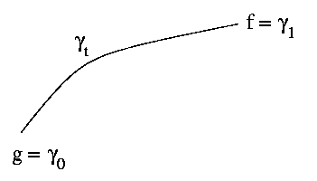
Figure 1: Path Connecting g and f
We assume that f(x) is a complicated expression (with x possibly high
dimensional) from which we want to sample. Due to the complexity of f(x)
we assume that there is no simple method for generating samples from f
but we assume that there is available a method for generating samples from
g.
It is intuitively clear how a path connecting the target distribution f
with the simpler distribution g may help by providing a way to arrive to
the target in little steps along the path. In the following sections we show
two examples of the application of this simple but powerful idea.
There are many ways of building paths between densities but there are two
special connections that have been proven useful, not only for generating
random variables with the computer but also in the general theory of
information geometry. I am of the opinion that the utility of the
exponential and mixture connections is just the tip of the iceberg. I think
that there is a whole unexplored geometric world lurking behind computer
sampling.
The Exponential Connection
A path can be obtained by mixing the loglikelihoods of two extreme
distributions,
|
log( gt(x)) = t log f(x) + (1-t)log g(x) - log Zt |
|
where Zt is a normalization constant. We can also write,
with,
This path is known as the exponential connection between the densities g
and f. The path is an exponential family with t as the natural
parameter and the loglikelihood ratio log(f(x)/g(x)) as sufficient
statistic. This connection provides a notion of a straight line in the space
of distributions that is diametrically opposed to the notion of straightness
provided by the mixture connection introduced next.
The Mixture Connection
Another path connecting the target density f to the easier to sample from
density g, is given by the mixture connection,
|
gt(x) = t f(x) + (1-t) g(x) |
|
This path provides an alternative notion of a straight line in the space of
distributions. Different ways of defining straightness give different ways
of defining curvature and parallelism for example.
Thermodynamic Integration
Thermodynamic integration is a technique that makes use of the exponential
connection for estimating the ratio of two normalization constants. The
problem of computing the ratio of two normalization constants appears in the
important problem of model selection or hypothesis testing. Suppose that we
want to compare two competing models M0, M1 for the available data
D. We need to compute the ratio of the two posterior probabilities for
the models. By Bayes' theorem we get,
|
log |
P(M0 | D)
P(M1 | D)
|
= log |
P(D|M0)
P(D|M1)
|
+ log |
p(M0)
p(M1)
|
|
|
where, p(Mi) are the prior probabilities for the two models. The
above expression is a recurrent head ache for the faithful Bayesians for two
reasons. First, the standard improper non informative priors can't be used
here. The ratio of infinities for the second term on the right is undefined
when improper priors are used. Second, it is not enough to know the
likelihood for the data up to a normalization constant since the first term
on the right needs the ratio of both normalization constants in order to
produce a definite numerical answer.
Let us then assume that the target density is only known up to a
proportionality constant, i.e.,
with,
unknown. Allow also the possibility of having g unnormalized, even though
this is less common, i.e. define,
which it is of course 1 when g is a proper density. The objective is to
compute,
|
| |
|
|
| |
|
| |
|
| |
|
| log |
ì
í
î
|
1
N
|
|
N
å
j = 1
|
|
h(xj)
g(xj)
|
ü
ý
ŷ
|
|
|
| |
|
where the x1,x2,ỳ are iid with density proportional to
g. In a few dimensions when g is very close in shape to h the
above approximation may work. In general, the simple importance sampling
approximation above, fails to produce useful estimates. The use of the
exponential connection can improve the estimates dramatically in the
following way. Define,
which is the normalization constant for the mixture of the log likelihoods of
h and g. Notice that the definition includes the extremes that we are
after Z0 and Z1. From,
|
Zt+e = |
ó
õ
|
|
æ
ç
è
|
h(x)
g(x)
|
ö
ṫ
ø
|
e
|
ht(x)g1-t(x) dx |
|
we obtain,
|
|
Zt+e
Zt
|
= < |
æ
ç
è
|
h(x)
g(x)
|
ö
ṫ
ø
|
e
|
> t |
|
where by the last notation we mean the expected value of what is inside the
brackets when x follows the exponential connection density with parameter
t. For values of e close to zero the sample means obtained by
using the Metropolis algorithm produce very accurate estimates of the ratios
for different values of t. Finally by climbing up the path we obtain,
|
|
Z1
Z0
|
= |
Z1/n
Z0
|
|
Z2/n
Z1/n
|
ỳ |
Z(n-1)/n
Z(n-2)/n
|
|
Z1
Z(n-1)/n
|
|
|
which is estimated as,
|
| |
|
|
|
|
n-1
å
i = 0
|
log < |
æ
ç
è
|
h(x)
g(x)
|
ö
ṫ
ø
|
1/n
|
> i/n |
| |
|
|
n-1
å
i = 0
|
log |
æ
ç
è
|
1
N
|
|
N
å
j = 1
|
|
æ
ç
è
|
h(xi,j)
g(xi,j)
|
ö
ṫ
ø
|
1/n
|
ö
ṫ
ø
|
|
|
| |
|
where xi,1,xi,2,ỳ, xi,N are sample from the exponential
connection with parameter i/n. Thus, in order to get the ratio we need to
implement a sequence of MCMCs.
It is also possible to get a good estimate of the ratio by running a single
MC but at the expense of having to generate from an equiprobable mixture of
exponential connections. Here is how: Write,
|
| |
|
|
|
|
lim
e®0
|
|
|
< |
æ
ç
è
|
h(x)
g(x)
|
ö
ṫ
ø
|
e
|
> t -1 |
e
|
|
| |
|
| < |
d
de
|
exp(elog |
h
g
|
) > t = < log |
æ
ç
è
|
h(x)
g(x)
|
ö
ṫ
ø
|
> t |
|
| |
|
from where we get,
|
logZt = |
ó
õ
|
t
0
|
< log |
h(x)
g(x)
|
> ldl+ logZ0 |
|
denoting the exponential connection with parameter l by
gl and interchanging the order of integration we obtain,
|
log |
Z1
Z0
|
= |
ó
õ
|
log |
h(x)
g(x)
|
|
é
ë
|
|
ó
õ
|
1
0
|
gl(x) dl |
ù
û
|
dx |
|
and by calling,
the continuous equiprobable mixture of the elements of the path connecting
f with g we can write,
|
log |
Z1
Z0
|
= < log |
h(x)
g(x)
|
> G* |
|
a very beautiful formula in its own very self and also useful. It says
something like
the log of the ratio of averages of two positive functions
equals the average of log of ratios
with respect to the average exponential connection
linking those two functions
The Plain Vanilla Thermodynamic Integrator
{
sum Ỳ 0
for j = 1,2,ỳ,N
{
u Ỳ unif(0,1)
x Ỳ sample gu by Metropolis
sum Ỳ sum + log[h(x)/g(x)]
}
return sum/N
}
In the above algorithm the metropolis steps can be dramatically improved by
starting from a previously observed sample from gt with t as
close as possible to the current u so that only a few iterations are
necessary.
The Full Monty-Carlos Method
This is a new, as far as I know previously unknown method, that allows to
sample from any f starting from any g. The simplest version of the
method works as long as the ratio of normalization constants of f and
g is known. If that ratio is unknown, it must first be
estimated by one of the methods of the previous sections.
A modification of the simpler version allows the freedom of using
unnormalized densities.
The idea is very simple and it exploits a simple but super useful property of
the mixture connection.
Theorem 1
Let,
|
gt(x) = t f(x) + (1-t) g(x) |
|
be the mixture connection between two fully normalized pdfs (or probability
mass functions) f and g. Then, for all values of x
|
gt+e(x) < |
æ
ç
è
|
1 + |
e
t
|
ö
ṫ
ø
|
gt(x) |
|
for all t and e so that the mixture parameters are always in
[0,1].
Proof: just write,
and consider two cases.
- Case I: f(x) £ g(x)
-
In this case it follows from the last equation that, l £ 1.
- Case II: f(x) > g(x)
-
For this case write the denominator in the last equation above as,
gt(x) = g(x)+t(f(x)-g(x)) and divide the numerator
and the denominator by (f(x)-g(x)) to obtain,
|
l = 1 + |
e
t + g(x)/(f(x)-g(x))
|
< 1 + |
e
t
|
|
|
Q.E.D.
The Monty-Carlos method makes use of this theorem in the following way. Start
by generating a sample from g = g0 then move (horizontally in the
picture) with a few metropolis iterations to get a sample from
g1/n. Then, try to climb up towards f as much as possible by
using the exact rejection constants provided by the previous theorem. When
the sample gets rejected then fall back to the last acceptance that assures
that the sample is from gk/n. This x is now used as an
initial value for metropolis to try to go one step forward to
g(k+1)/n. Continue in this way until arriving at f.
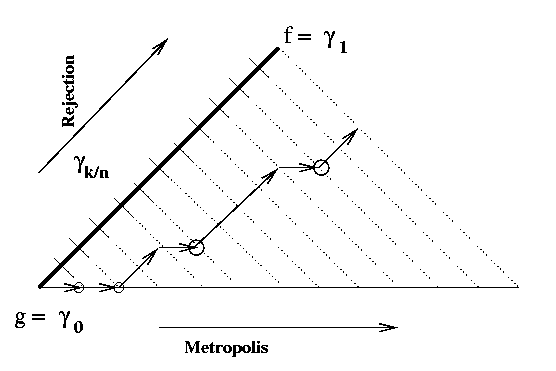
Figure 2: The Full Monty-Carlos Method
When n is small and g is close to f the method can be used for
generating independent samples from f. For really complicated high
dimensional f a high value for n is needed and there is no guarantee
that g is close to f. In such cases, the method can be used for
producing a single sample from f and after that continue with a version
of metropolis but now knowing that metropolis has converged.
In order to provide a short description of the algorithm will make use of two
functions:
- Met(x,t,Stop_crit)
- Returns a sample from gt starting from
x using the metropolis algorithm with a given stopping criterion
(e.g. maximum number of iterations).
- Climb(x,k,n)
- Returns an integer kḃ with k £ kḃ £ n. The
sample x from gk/n is pushed-up as high as possible until it
gets rejected at gkḃ/n.
The Full Monty-Carlos Algorithm
{
x Ỳ sample from g(·)
k Ỳ 1
while (k < n)
{
x Ỳ Met(x,k/n,Stop_crit)
k Ỳ Climb(x,k,n)
}
Return x
}
Met(x,t,Stop_crit)
{
until (Stop_crit)
{
y Ỳ sample g(·)
u Ỳ unif(0,1)
if u < min(1, [(gt(y))/(gt(x))])
then x Ỳ y
}
Return x
}
Climb(x,k,n)
{
j Ỳ 0
u Ỳ unif(0,1)
while ( k+j < n ) AND
|
|
æ
ç
è
|
u* |
é
ê
ë
|
1+ |
1
k+j-1
|
ù
ú
û
|
*g(k+j-1)/n(x) < g(k+j)/n(x) |
ö
ṫ
ø
|
|
|
{
u Ỳ unif(0,1)
j Ỳ j+1
}
Return k+j
}
0.1 The Full-Monty Without Normalization Constants
If f and g are only known up to normalization constants
the method works if we just change the Climb function to:
Climb(x,k,n)
{
j Ỳ 0
u Ỳ sample from exp(1)
while ( k+j < n ) AND
|
|
æ
ç
è
|
u < log |
æ
ç
è
|
(k+j)g(k+j-1)/n(x)
(k+j-1)g(k+j)/n(x)
|
ö
ṫ
ø
|
ö
ṫ
ø
|
|
|
{
u Ỳ sample from exp(1)
j Ỳ j+1
}
Return k+j
}
The fact that it works follows from the following (well known)
theorem:
Lemma 1
For a nonnegative function h(x) the algorithm,
{
Repeat
{
x Ỳ sample from g()
u Ỳ sample from exp(1)
}
Until h(x) £ u
Return x
}
produces a sample with density
proof:
For any borel set B we have,
|
| |
|
|
|
|
P[X Î B, U ġ h(X)]
P[U ġ h(X)]
|
|
| |
|
|
|
|
|
ó
õ
|
B
|
|
ó
õ
|
ċ
y = h(x)
|
g(x)exp(-y) dy dx |
|
|
| |
|
| |
|
|
| |
|
File translated from TEX by TTH, version 2.32.
On 5 Jul 1999, 22:59.