Lecture VII

An Introduction to Markov Chain Monte Carlo

Lecture VII

Abstract

The Hybrid Monte Carlo Method: Hamiltonian Dynamics, Liouville's Theorem, Leapfrog Discretization. The Non-Reversible Directed Metropolis.

Adding Momentum Variables

Recall that to sample from,

f(x) =

exp{ -(-logf(x)) }

we use the Metropolis algorithm with energy function as -logf(x). As it will be seen later, it is useful to think of the x Î Rⁿ only as the position variables q = (q₁,ź,q_n) so that the log-likelihood plays the role of a potential energy. By introducing an independent extra set of momentum variables p = (p₁,ź,p_n) with i.i.d. standard Gaussian distributions we can add a kinetic term to the potential to produce a full Hamiltonian (energy) function on a ficticious phase-space,

H(q,p) = -logf(q) +

ĺ
i

p_i²

The Cannonical distribution associated to this Hamiltonian is,

p(q,p) =

Z_H

exp{ -H(q,p) }

and we can sample from it by using a combination of Gibbs and Metropolis and finally discard the momentum variables to show only the position variables that by construction are now comming from the correct marginal distribution f(q).

The extra burden of enlarging the dimensions of the sampling space to then through them away at the end, looks like a complete waste, but there is ofcourse a benefit associated to this procedure. What is gained by adding the momentum variables is a way to efficiently explore large regions of phase-space by simmulating the Hamiltonian dynamics in ficticious time. As it is shown in the next sections, by following the dynamical path in phase-space, we can propose cadidate moves that are far away from the current state but that still have a substantial chance of being accepted.

The validity of the Hybrid Monte Carlo Method rests on three standard properties of Hamiltonian dynamics:

Time reversibility, i.e. invariance under tŽ -t,pŽ -p.
Conservation of Energy, i.e. H(q,p) is the same for all times.
Liouville's theorem, i.e. conservation of phase-space volumes.

We look at each of these properties in the next sections.

Hamiltonian Dynamics in Ficticious Time

Let us introduce a ficticious time t along which we assume the system is evolving according to Hamilton's equations derived in lecture I. In component form they are,

dq_i

.
q_i

śH

śp_i

= p_i

dp_i

.
p_i

śH

śq_i

ślogf(q)

śq_i

where for the rightmost hand-side we have replaced the specific Hamiltonian defined in the previous section. It is interesting to notice that in this ficticious dynamics the field of forces is supplied by the score function (i.e. the derivatives of the loglikelihood).

Time Reversivility

The above system of equations is invariant under the transformations,

-t = t˘

-p = p˘

q = q˘

To see it, first notice that the Hamiltonian is the same, i.e.,

H˘(q˘,p˘)

-logf(q˘) +

ĺ
i

(p˘_i)²

-logf(q) +

ĺ
i

p_i²

H(q,p)

and the equations are also the same,

dq˘

dt˘

śH˘

śp˘

= -

śH

śp

dp˘

dt˘

= -

śH˘

śq˘

śH

śq

This is usually stated by saying that the equations of Classical Mechanics are blind to the direction of time. The equations can not tell if the movie of the universe is being run forwards or backwards! I don't know which universe classical mechanics is trying to describe... certainly not mine! This is the tip of the iceberg of the so called problem of time. Quantum theory suffers the same ache. The appearance of the arrow of time has been related to the second law of thermodynamics (MaxEnt^TM), the expansion of the universe, the Big!, and even conciousness!. I have humbly (yeh, right..) proposed a connection to uncertainty in the measurement of location.

Conservation of Energy

With the help of Hamilton's equations we can compute the rate of change with respect to time (i.e. the time derivative) of any quantity F(q,p) defined as a function on phase-space. By the chain rule,

F(q,p) =

śF

śq

.
q

śF

śp

.
p

were we have suppressed the summation over the coordinates by denoting the innerproduct of vectors with a plain product. Replacing Hamilton's equations we get,

F(q,p) =

śF

śq

śH

śp

śF

śp

śH

śq

ş { H,F}

the last formula is known as the Poisson bracket (it is a Lie product). The derivative wrt time of any function F is then obtained by computing the Poisson bracket of F with the Hamiltonian for the system H. The Hamiltonian tells how things change with time. When F = H we get,

H(q,p) = 0

and therefore things may change but energy doesn't. H i.e. total energy is a constant of time.

Liouville's Theorem

Take a piece of phase-space of some volume v. Now think of each of the points inside this volume as different systems with the same Hamiltonian but with different initial conditions. Let time go and the systems evolve according to Hamilton's equations. After some time the points initially inside the volume v would be spread all over. However, the equations of movement assure that the volume of phase-space covered by these points, is the same at all times. That is Liouville's theorem and that is what we now prove.

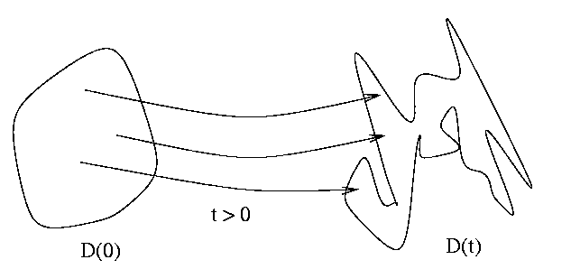
Take an arbitrary time t₀ and an arbitrary region of phase-space, D₀. Without loss of generality assume this time to be zero. Let D(t) be the region of phase-space at time t occupied by the points that at time zero were in D(0) = D₀. As in the picture.

Figure 1: Illustration of Liouville's Theorem

The volume of D(t) is,

v(t) =

ó
ő

D(t)

dq˘dp˘ =

ó
ő

D(0)

det

(I+tM) dq dp + O(t)

where we have used the change of variables,

q˘

q + t

.
q

+ o(t)

p˘

p + t

.
p

+ o(t)

with the little o's holding as tŽ 0. The matrix M is the part of the Jacobian with the derivatives of [q\dot] and [p\dot]. We have,

det

(I+tM) = 1 + ttr M + o(t)

where tr is the trace and we have,

tr M =

.
q

śq

.
p

śp

śq

ć
ç
č

śH

śp

ö
÷
ř

śp

ć
ç
č

śH

śq

ö
÷
ř

= 0

where we have replaced Hamilton's equations and assumed continuity for the second order partial derivatives of H in order to have the equality of the mixed partials. Thus, we can write,

v(t) =

ó
ő

D(0)

(1+0) dq dp + o(t) = v(0) + o(t)

from where we obtain,

v(t)

ę
ę
ę

= 0

and since t₀ = 0 was arbitrary we have shown that the derivative is zero for all times. Hence, the volume is a constant of time.

Leapfrog Discretization

To simmulate the Hamiltonian dynamics we need to discretize the equations of motion and in general, unless we are carefull, the error introduced by the discretization destroys time reversibility and the preservation of volumes which are both needed for metropolis to work without changes. The so called leapfrog discretization has the desired properties. Leapfrog updates the coordinates q_i, p_i in three steps. First it takes a little half step for the momentum,

^
p

(t+e/2) =

^
p

(t) +

ślogf

śq_i

(

^
q

(t))

then it takes a full step for the position,

^
q

(t+e) =

^
q

(t) +e

^
p

(t+e/2)

and finally the other half step for the momentum,

^
p

(t+e) =

^
p

(t+e/2) +

ślogf

śq_i

(

^
q

(t+e))

leap-Leapity-leap that's why it's called leapfrog. At the end of the three steps we obtain an approximation to the values of position and momentum at time t+e from their corresponding values at time t. As it can be readily check by simple inspection, the leapfrog discretization has the following necessary property:

it allmost preserves H, in fact to order O(e²).
it preserves volumes since the above are just shear transformations.
it is time reversible.

The Hybrid Monte Carlo Method

The Hybrid Monte Carlo Method is plain vanilla metropolis in phase-space with the following proposal distribution:

Choose random direction of time, i.e., with probability 1/2 simulate the dynamics forward or backward in time.
Given a current state (q,p) = (q(0),p(0)) of energy H. Perform a random number L of leapfrog steps with (possibly random) small stepsize e in the random direction choosen above. This produces a candidate state (q˘,p˘) with energy H˘.

the candidate state is then accepted with the usual metropolis probability of acceptance,

min

{1,exp[ -(H˘- H) ]}

The probability of acceptance can be made arbitrarily close to one by decreasing the stepsize of the discretization. Recall, that the value of the energy reamins constant along the trajectory of the system in phase-space. The discretization beeing an inexact simulation of the dynamics of the system, introduces a small error so that H˘-H is not equal to zero but not large.

Hybrid Monte Carlo Works

The validity of the algorithm follows from the symmetry of the proposal distribution introduced above. To see that the proposal distribution is in fact symmetric consider the probability of proposing a small region D˘ given that the current point is known to be in a small region D of volume dv in phase-space. Since, the simulated Hamiltonian dynamics with leapfrog discretization is invariant under time reversals and it preserves volumes it follows that D˘ has volume dv as well and the chance of proposing a state in D starting from D˘ is the same as the chance of proposing D˘ from D.

The benefit of following the trajectory of the system in phase-space is the fact that we can explore quickly regions that are far away from the current state eliminating the random walk aspect of the chain improving mixing and producing more accurate estimates.

File translated from T_EX by T_TH, version 2.32.
On 5 Jul 1999, 22:59.