Lecture VI

An Introduction to Markov Chain Monte Carlo

Lecture VI

Abstract

Neural Networks as a way to specify nonparametric regression and classification models.

Feed Forward Neural Nets Models

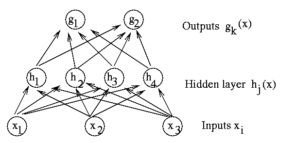
Feed forward Neural Nets are also known as multilayer perceptrons or backpropagation networks. The figure shows a network with a layer of 4 hidden units.

Figure 1: A Feed Forward Network

The outputs are computed from the following formulas,

g_k(x)

b_k +

å
j

v_jk h_j(x)

(1)

h_j(x)

tanh(a_j +

å
i

u_ij x_i )

(2)

where {a_j},{b_k},{u_ij},{v_jk} are the parameters of the network. The parameters with one index are known as biases and those with two indeces are known as weights. We assume that x = (x₁,¼,x_d) Î R^d, h(x) = (h₁(x),¼,h_l(x)) Î R^l, g(x) = (g₁(x),¼,g_p(x)) Î R^p. The hyperbolic tangent,

tanh(z) =

sinh(z)

cosh(z)

e^z-e^-z

e^z+e^-z

1-e^-2z

1+e^-2z

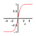
Figure 2: Hyperbolic Tangent

is an example of a sigmoid function. A sigmoid is a non-linear function, s(z), that goes through the origin, approaches +1 as z®¥ and approaches -1 as z® -¥.

It is known since 1989 (only) that as the number of hidden units increases, any function defined on a compact set can be approximated by linear combinations of sigmoids.

Multilayer perceptrons are often used as flexible models for nonparametric regression and classification. Given data,

(x⁽¹⁾,y⁽¹⁾), (x⁽²⁾,y⁽²⁾),¼, (x⁽ⁿ⁾,y⁽ⁿ⁾)

with,

y^(k) = g(x^(k),q) + e^(k)

where

e⁽¹⁾,e⁽²⁾,¼,e⁽ⁿ⁾ are iid with Ee^(k) = 0

Hence, the g is the regression of y on x, i.e.,

E(y | x,q) = g(x,q) with q Î Q

The multilayer perceptrons provide a practical way to define the functions g with high dimensional parameter spaces Q. We take q = { {a_j},{b_k},{u_ij},{v_jk} }. The objective is to find the predictive distribution of a new target vector y, given the examples D = ((x⁽¹⁾,y⁽¹⁾), (x⁽²⁾,y⁽²⁾),¼,(x⁽ⁿ⁾,y⁽ⁿ⁾)) and the new vector of inputs x, i.e.,

f(y | x, D) =

ó
õ

f(y | x, q) p(q| D) dq

Under the assumption of quadratic loss, the best guess for y will be its mean,

^
y

= E(y | x,D) =

ó
õ

g(x,q) p(q|D) dq

These estimates can be approximated by MCMC by sampling q⁽¹⁾,¼,q^(N) from the posterior and then computing empirical averages,

^
y

N
å
j = 1

g(x,q^(j))

Useful Priors on Feed Forward Networks

In the absence of specific information, the following assumptions about the prior p(q) are reasonable,

The components of q are independent and symmetric about 0.
Parameters of the same kind have the same a priori distributions, i.e.,

a₁,a₂,¼ iid

b₁,b₂,¼ iid

u_1j,u_2j,¼ iid for all j

v_1k,v_2k,¼ iid for all k

With these assumptions if var_p(v_jk) = l^-1s²_v < ¥ then by the Central Limit Theorem, as l® ¥ the prior on the output units converges to a Gaussian process. Gaussian processess are characterized by their covariance functions and they are often considered innadequate for modeling complex inter-dependence of the outputs. To avoid the Gaussian trap, it is convenient to use a priori distributions for the components of q that have infinite variance.

A practical choice (used by Neal) is to take,

v_jk as t-distribution µ

æ
ç
è

1 +

v_jk²

as_v²

ö
÷
ø

-(a+1)/2

with 0 < a < 2

Furthermore, if the we take s_v = w_v l^-1/a then the resulting prior will converge as l®¥ to a symmetric stable process of index a.

Recall that Z₁,Z₂,¼,Z_n iid with distribution symmetric about 0 are said to be stable of index a if

Z₁ + ¼+ Z_n

n^1/a

has the same law as Z₁

A distribution is said to be in the domain of attraction of a stable law if properly normalized sums of independent observations from this distribution, converge in law to a stable distribution. Hence, distributions with finite variance are in the domain of attraction of the Gaussians. It is also well known that distributions with tails going to zero as |x|^-(a+1) as |x|®¥ are in the domain of attraction of stable laws of index a which justifies the choice of t-dist above.

Postulating an Energy for the Net

An alternative approach without priors (apparently...) is to postulate directly and Energy function for the network, e. g,

E(q,g) =

n
å
k = 1

L(y^(k),g(x^(k),q)) + g||q||²

where L(y,z) is the assumed loss when we estimate y with z. Typical choices are L(y,z) = R(||y-z||) for some nondecreasing function R and some norm ||·||. Then choose q to minimize this Energy function. Often, the smoothness parameter g > 0 is chosen by Cross-Validation or by plain trial and error.

For complicated multi modal energy functions, a combination of simulated annealing with a classical gradient method (such as conjugate gradients) have been the most successful.

File translated from T_EX by T_TH, version 2.32.
On 5 Jul 1999, 22:59.