Lecture IV

An Introduction to Markov Chain Monte Carlo

Lecture IV
Lecture IV
Abstract
The Rejection and Acceptance Complement Methods.
Exact Sampling Methods
The Metropolis algorithm and its variants are great, for they can be used to
generate ergodic Markov chains with, in principle, any pre specified
stationary distribution. Just choose an arbitrary starting point and
eventually the chain will begin sampling from its stationary distribution.
The problem is, of course, that (usually) we can't be 100% sure about when
this will happen. Exact sampling methods, when available, are therefore more
reliable and, often more efficient than MCMC methods. For this reason MCMC
sampling is almost always used in combination with exact methods. This is
specially true for the Gibbs sampler where we need to generate from the
full conditionals. What exact method to use depends on the particular
problem. There are literally hundreds of methods available. The current
bible is Devroye's book which is
unfortunately not available online. Besides the only truly universal
exact generator (the inverse cdf method introduced in
lecture I) the most flexible exact algorithm is
the rejection method.
The Rejection Method
The idea, I think first implemented by Von Neumann, is very simple. To
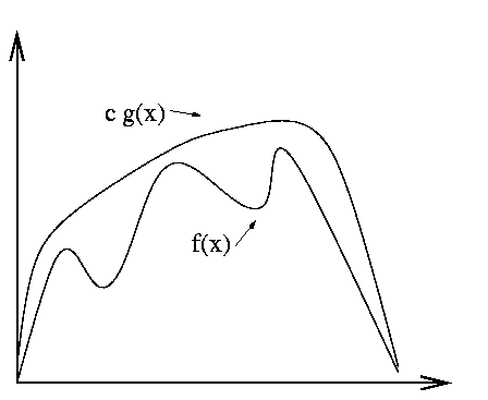
sample from f(x) find another simpler density g(x) from which you
know how to sample and such that c g(x) ł f(x) for some c > 1 (we
say that c g envelopes f). Like in the following picture:

Then generate uniformly under the graph of
the envelope and accept only samples that fall under the graph of f.
In other words reject a sample if it falls in between the envelope
and the function f.
Copying from the bible:
Theorem 1
If f and g are densities on Rp with, f(x) Ł c g(x) for
all x Î Rp, some c ł 1. Then the following algorithm
The Rejection Method
{
REPEAT
{
x ¬ sample from g
u ¬ unif(0,1)
y ¬ c [g(x)/f(x)]
}
UNTIL uy Ł 1
RETURN x
}
will produce a sample X = x with density f(x).
Proof: Consider the following two lemmas
Lemma 1
Let X be a random p-vector with density f(x). Let U be a
uniform(0,1) r.v. independent of X, and let c > 0. Then,
- I.
- (X,c U f(X)) is uniform on,
A = {(x,u) : x Î Rp, 0 Ł u Ł c f(x) }
- II.
- If (X,U) is uniform on A, then X has density f(x).
Proof:
- I.
- Let B Ě A, then
|
| |
|
|
|
|
ó
ő
|
P[(x,c U f(x)) Î B | X = x ] f(x) dx |
| |
|
|
|
ó
ő
|
|
ě
í
î
|
|
ó
ő
|
Bx = {u:(x,u) Î B}
|
|
1
c f(x)
|
du |
ü
ý
ţ
|
f(x) dx |
| |
|
|
| |
|
where the second equality follows from Tonelli's theorem, the independence
of X and U and the fact that cf(x)U is uniform(0,cf(x)).
But,
|
|A| = |
ó
ő
|
A
|
du dx = |
ó
ő
|
Rd
|
( |
ó
ő
|
cf(x)
0
|
du)dx = c |
|
thus, for any B Ě A measurable we have,
|
P( (X,cUf(X)) Î B ) = |
|B|
|A|
|
|
|
which means that (X,cUf(X)) is uniform on A.
- II.
- We just need to show that, "B measurable,
P[X Î B] = ňB f(x) dx. But,
|
| |
|
|
|
P[ X Î B, 0 Ł U Ł c f(X) ] |
| |
|
|
P[(X,U) Î B1 = {(x,u):x Î B, 0 Ł u Ł cf(x)}] |
| |
|
| |
|
|
1
c
|
|
ó
ő
|
B
|
c f(x) dx = |
ó
ő
|
B
|
f(x) dx. |
|
| |
|
Lemma 2
Let X1,X2,Ľ be iid vectors in Rp. Let A Ě Rp s.t.
P[X Î A] = a > 0. Let Y be the first Xi Î A. Then,
"B Ě Rp measurable,
Moreover, if X1 is uniform on A0 É A then Y is uniform on
A.
Proof:
|
| |
|
|
|
|
Ą
ĺ
i = 1
|
P[X1\not Î A,Ľ, Xi-1\not Î A,Xi Î B |
Ç
| A ] |
| |
|
|
|
Ą
ĺ
i = 1
|
(i-a)i-1 P[X1 Î B |
Ç
| A] |
| |
|
|
| |
|
Also, if X1 is uniform on A0 É A then for all measurable B,
|
| |
|
|
|
|
P[X1 Î ABA0)
a
|
= |
|ABA0| / |A0|
|A0A| / |A0|
|
|
| |
|
|
| |
|
therefore, Y is uniform on A.
We are now ready for the Theorem.
Proof: (that the Rejection Method is valid). In the first line
the algorithm generates (by Lemma 1, I) (X,cUg(X)) uniform on
C = {(x,u): x Î Rp, 0 Ł u Ł c g(x) }. However at
exit time (by Lemma 2), (X,cUg(X)) is uniform on
C = {(x,u): x Î Rp, 0 Ł u Ł f(x) }.
Notice that, by the assumption that f(x) Ł cg(x)
(i.e. that g envelopes f), C É A.
Thus, (by Lemma 1, II) X has density f(x).
Best g is f itself
Let N be the number of pairs (x,u) generated by the rejection
algorithm to exit. We have,
|
| |
|
|
|
P[ reject at least (i-1) pairs ] |
| |
|
| P[ UY ł 1 ]i-1 = (1-a)i-1 |
|
| |
|
where,
|
| |
|
|
|
P[ U c |
g(X)
f(X)
|
Ł 1 ] = |
ó
ő
|
P[Ucg(x) Ł f(x)] g(x)] dx |
| |
|
|
ó
ő
|
|
f(x)
c g(x)
|
g(x) dx = |
1
c
|
. |
|
| |
|
The expected number of pairs generated by the algorithm is, < N > where,
|
< N > = |
Ą
ĺ
i = 1
|
P[N ł i] = |
Ą
ĺ
i = 1
|
(1-a)i-1 = |
1
1-(1-a)
|
= |
1
a
|
= c |
|
Thus, c is the expected number of rejections and therefore it should be
kept as small as possible, i.e. as close as possible to its minimum value
of 1. Since, f(x) Ł c g(x), in order for c to be small g must be
close to f.
Example: To sample from the standard Gaussian we can use the
rejection method with g as the Laplace distribution. Notice that,
|
f(x) = (2p)-1/2 exp(-x2/2) |
|
and in order to get an upper bound for f we need a lower bound
for the energy, i.e. for x2/2. But that follows easily from,
|
|
1
2
|
(|x| - 1)2 = |
x2
2
|
+ |
1
2
|
- |x| ł 0 |
|
from where we get,
|
exp(-x2/2) Ł exp( |
1
2
|
- |x|) = (2p)1/2 |
ć
ç
č
|
2e
p
|
ö
÷
ř
|
1/2
|
|
ć
ç
č
|
1
2
|
exp(-|x|) |
ö
÷
ř
|
|
|
the last term in parenthesis above, is the density of the Laplace
distribution which the above inequality shows to envelope the N(0,1)
with,
|
c = |
ć
ç
č
|
2e
p
|
ö
÷
ř
|
1/2
|
» 1.3155 |
|
Javascript Demo Implementation of the above in Javascript.
Solution by Ke Yang
There are several variations of the rejection method in the bible.
One fairly general method that never rejects any samples is:
The Acceptance Complement Method
Suppose that we don't know how to envelope f but,
with, f1(x) ł 0, f2(x) ł 0 and f1(x) ł g(x) where
g is a density. Furthermore suppose that we know how to sample from
g and from f2 (properly normalized), then,
The Acceptance Complement Method
{
x ¬ sample from g
u ¬ unif(0,1)
IF u > f1(x) / g(x) THEN x ¬ sample from f2/ňf2
RETURN x
}
Theorem 2
X = x is a sample from f.
Proof: Let a = ňf2 and suppose that Y has density g. We
have,
|
| |
|
|
|
P[Y Î B, U Ł |
f1(Y)
g(Y)
|
] +P[U > |
f1(Y)
g(Y)
|
] |
ó
ő
|
B
|
f2(x) dx / a |
| |
|
|
|
ó
ő
|
B
|
|
f1(x)
g(x)
|
g(x) dx + |
ć
ç
č
|
1 - |
ó
ő
|
|
f1(y)
g(y)
|
g(y) dy |
ö
÷
ř
|
|
ó
ő
|
B
|
f2/a |
| |
|
|
ó
ő
|
B
|
f1 + |
ó
ő
|
B
|
f2 = |
ó
ő
|
B
|
f |
|
| |
|
Example: f1(x) = min{f(x),g(x)} and f2(x) = (f(x)-g(x))+.
Then, clearly f1(x) Ł g(x) and f(x) = f1(x) + f2(x). So if
we know how to sample from g and f2, we are done.
Another useful general split is available for almost flat densities on
[-1,1], i.e. densities f(x) such that,
then we may take,
|
| |
|
|
| |
|
|
f(x) - (M - |
1
2
|
), with M = |
sup
| f(x) |
| |
|
|
| |
|
which works since g and f2 are proportional to densities uniform on
[-1,1] (so easy to sample from). That f1 is bounded above by g just
follows from the almost flat condition and that f1 > 0 follows from the
fact that,
|
0 Ł |
inf
| f(x) Ł |
1
2
|
Ł |
sup
| f(x) Ł 1 |
|
Hence, the method can be used to generate from many densities symmetric about
with a single mode at 0, for which M = f(0) and inf f = f(1). For example
we can generate from the truncated Cauchy for |x| Ł 1. We have,
|
f(x) = |
2
p(1+x2)
|
for |x| Ł 1 |
|
which is almost flat since 2/p- 1/p = 1/p » 0.318 < 0.5. Using
the property that 1/X is Cauchy when X is Cauchy we can generate a
complete Cauchy by just using the Acceptance Complement Method to generate
from the truncated Cauchy and then with probability 1/2 return 1/X
instead of X.
Example: Javascript implementation of the Cauchy with the above method.
A Trivial Perfect MCMC Method
If there is available a good envelope for f then the rejection method is
preferable to asymptotic methods based on Markov chains. The problem is that
often good envelopes are not easy to find. A bad envelope can be easier to
find and still be useful when combined with a Markov chain method. For
example it may be possible to show that f(x) Ł 10000 g(x) which means
that we can use the rejection method but expect to generate, on the average,
10000 (X,U) pairs before accepting one vector X. In this case we can
still use the rejection method to generate a single observation of X which
is warranted to have the correct density f. Then, use the observation
generated by the rejection method as the initial point for a Markov chain
method with statitionary distribution f and harvest the complete path of
the chain that is now sampling from its asymptotic distribution.
File translated from TEX by TTH, version 2.32.
On 5 Jul 1999, 22:59.
