Lecture II

An Introduction to Markov Chain Monte Carlo

Lecture II
Lecture II
Abstract
Statistical Physics (part 2), the original Metropolis Algorithm,
Simulated Annealing.
Phase Space
It is convenient to visualize a mechanical system as a point in the
6N dimensional space (q,p) of all the positions and momenta
of all the N particles.

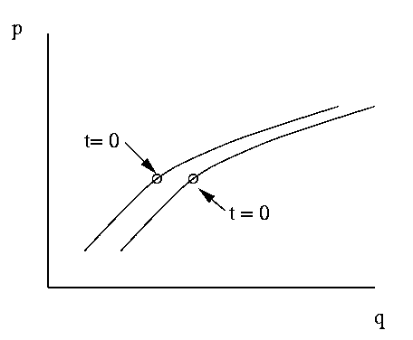
Figure 1: Two trajectories in phase-space
Due to the complexity of macroscopic systems (N ~ 1024) it
was necessary to abandon determinism and use statistics to describe
the system. The predictions of statistical physics are expected to hold
only on the average.
Instead of the precise initial conditions (which are unknown), statistical
physics describes the system by a probability distribution over phase space,
r(q,p) for t = 0. As it will be seen later, Hamilton's equations imply
the conservation, at all time, of this initial distribution. This is the
famous, Liouville's theorem. The determination of r is then the first
step.
Maxwell-Boltzmann-Gibbs Distribution
Different forms for r are found to be needed depending
on the particular data available about the system. We will be
concerned only with the so called canonical distribution.
We assume that the system is not isolated but in thermal equilibrium
with a heat bath at constant temperature T. Statistically this
is equivalent to the assumption that the average energy of the molecules
is constant. The novel idea of Boltzmann was to discretize phase-space
to find the most likely distribution for r.
Each particle has a definite position and momentum. Subdivide the positions
and momentums for each particle into m (6 dimensional) cells of equal size.
Assume that these cells are small enough so that the value of the energy
within each cell is approximately constant. Let Ej be the energy in the
j-th cell. Assume further that the cells, even though small, they are still
big enough to accommodate lots of particles inside. These are reasonable
assumptions justified by the smallness of atomic dimensions ( ~ 10-8
cm), the size of typical N and the smoothness of energy surfaces. This
discretization of the phase-space for each molecule into m equal size
cells induces a discretization of the phase-space of the system into,
mN equal size cells. With the help of this discretization, the
state s of the system is specified by,
indicating the cell number for each of the N particles. If the
particles are assumed to be identical and indistinguishable, then
permutations of the molecules with a given cell number have no
physical consequences. All it matters is how many molecules end
up in each of the cells and not which ones did. Thus, the actual
set of distinguishable physical states is much smaller than mN
it is,
corresponding to the number of ways of splitting N into the m
cells. There are,
ways of throwing the N molecules into the m cells in such a
way that n1 of them are in the first cell, n2 in the
second cell, etc. If we assume a priori that the molecules have
equal chance of ending in any of the cells then the number of ways
can be turned into a probability for the state s = (n1,Ľ,nm),
|
P = |
N!
n1! n2!Ľnm!
|
×constant |
|
Hence, the most likely distribution of balls among the cells is the
one that maximizes this probability subject to whatever is known about
the system. When the temperature is all we know we maximize P subject
to the constraint that the average energy is fixed at kT. Where
k is a phenomenological (not fundamental) constant needed to change the
units from ergs (units of energy) to degrees (usual units for
temperature). It is known as the Boltzmann constant and it is about,
|
k = 1.380 ×10⁻¹⁴ ergs per degree centigrade |
|
Using the fact that N and the nj are large we can use
Stirling's approximation,
to get,
|
| |
|
|
|
NlogN - |
ĺ
j
|
( njlognj - nj) + constant |
| |
|
| -N |
ĺ
j
|
pj log pj + constant |
|
| |
|
where,
Thus, P is the probability of observing the probability distribution
(p1,Ľ,pm). A probability of a probability... A prior!
Known as an entropic prior, for the quantity in the exponent (sans N) is
the famous expression for the entropy of a probability distribution.
If we treat the pj as if they were continuous variables we can
obtain the most likely a priori distribution by solving,
Using Lagrange multipliers for the constraints we can find the
maximum by maximizing,
|
L = |
ĺ
j
|
pj log pj - a- |
ĺ
j
|
pj- b |
ĺ
j
|
pjEj |
|
Taking derivatives,
|
|
¶L
¶pi
|
= 0 Ţlog pi - 1 -bEi -a = 0 |
|
from where we get,
where the normalization constant,
is known as the partition function. In order to satisfy the constraint of
average energy we need to take,
|
|
|
» |
ó
ő
|
Ą
0
|
E be-bE dE = k T |
|
and since the middle integral is the mean of the exponential distribution
we get,
The Original Metropolis Algorithm: Circa 1953
It was proposed as an algorithm to simulate the evolution of a system in a
heat bath towards thermal equilibrium.
From a given state i of energy Ei, generate a new state
j of energy Ej by a small perturbation, e.g. changing one of the
position coordinates of one of the particles a little. If the new
proposed state j has smaller energy than the initial state i then
make j the new current state, otherwise accept state j with probability,
|
Aij(T) = exp(-(Ej-Ei)/kT) |
|
where T is the temperature of the heat bath. After a (possibly) large number
of iterations we would expect the algorithm to visit states of different
energies according to the canonical distribution. In fact this can be
rigorously justified by showing that the sequence of states visited by
the algorithm forms an ergodic Markov Chain with the canonical distribution
as the stationary distribution for the chain.
Let, us get closer to the theory of Markov Chains by using the
usual notation. Define,
|
Xt = state of the system at time t |
|
The one step transition probabilities for the Metropolis (like) algorithm
are,
|
pij(T) = P[Xt+1 = j | Xt = i] = |
ě
ď
í
ď
î
|
|
|
|
|
where,
|
| |
|
|
|
prob. of generating j from i |
| |
|
| prob. of accepting j from i |
|
| |
|
The acceptance Metropolis probabilities can be written as,
|
Aij(T) = exp(-(Ej-Ei)+/kT) |
|
where,
Any, probability distribution p over the set of states satisfying
the reversibility condition known as detailed balance,
will be a stationary distribution for the Markov Chain with transition
probabilities pij. This can be easily seen by adding over j both
sides of the previous equation,
It can be readily checked that when the generating probabilities are
symmetric in i and j i.e. when,
we have detailed balance with,
i.e. the canonical distribution. Just consider each of the cases
separately. It is obviously true when i = j and for i ą j with Ei < Ej the detailed balance condition reduces to the simple identity,
|
exp(-(Ej-Ei)/kT) exp(-Ei/kT) = exp(-Ej/kT) |
|
the other case interchanges i with j, which is also obviously true. This
does not show, however that the chain is ergodic, i.e. that the distribution
of Xt will converge to the stationary canonical distribution.
Simulated Annealing
Annealing is a physical process often used in practice to get rid of cracks
and impurities from a solid in order to increase its strength. This is done
by first heating the solid until it melts and then slowly decreasing the
temperature to allow the particles to re-arrange themselves in the state of
lowest possible energy (ground state). The opposite of annealing is known as
quenching. The solid is melted but then the temperature is quickly lowered so
that the particles get frozen in a local minimum for the energy ( meta-stable
state). It is convenient to think of annealing as a way of using nature to
solve a minimization problem in billions of variables. The annealing process
is simulated by the Metropolis algorithm when we take a sequence of slowly
decreasing temperatures converging to 0. If we run the Metropolis algorithm
with each value of the temperature for a long time until it reaches the
asymptotic cannonical distribution, then in the limit when the temperature
approaches 0 the system will be found on state i with probability,
|
| |
|
|
| |
|
|
lim
T® 0
|
|
ĺ
j
|
exp |
ě
í
î
|
|
E*-Ei
kT
|
ü
ý
ţ
|
|
|
|
| |
|
where,
|
E* = |
min
i
|
Ei = Global min of energy |
|
Thus, the exponents (in the above ratios) are always either zero or
negative. In the limit when T® 0 the terms with negative
exponents disappear and we get,
|
|
lim
T® 0
|
pi(T) = |
ě
ď
ď
í
ď
ď
î
|
|
|
|
|
where,
Thus, limT® 0pi(T) is uniformly distributed over the
set of states of global minimum energy!
Simulated annealing is one of the few known algorithms assuring
convergence to a global minimum. It is often used in combination with
efficient steepest descent methods, such as conjugate gradients, as a way for
avoiding getting trap in local minima. This is what the theory says but in
practice the performance of annealing depends primarily on the cooling
schedule, i.e. how exactly is the temperature decreased and second on the
stopping criterion, i.e. how it is decided to stop the algorithm, for example
how close to zero is the temperature allowed to go before stopping.
File translated from TEX by TTH, version 2.32.
On 5 Jul 1999, 22:59.
