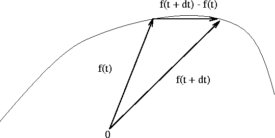
The length of a space curve can be computed by noticing that when
dt is close to zero then the length of the vector connecting f(t)
with f(t+dt) is close to the arc length, i.e.
 |
| Multiplying and dividing by "dt" we get |
> # that
     | f(t + dt) - f(t) |      | df(t) |
     | ---------------- | dt = | ----- | dt = "Arclength from t to t+dt"
     |        dt        |      |  dt   |
| Recall that the magnitud of the velocity vector is the speed at which the particle is moving in the direction tangent to its trajectory. So, the above equation indicates that the amount of space traveled is just (speed)*(time). Hence, to compute the total space traveled by the particle with trajectory f(t) during the interval of time from t=a to t=b, all we need to do is to add from t=a to t=b the above formula. i.e. |
> # formula
                                        b
                                        /
                                       |  | df(t) |
                             Length =  |  | ----- | dt
                                       |  |  dt   |
                                      /
                                      a
Clearly the length of a space curve can be computed independently of
the coordinate system used to describe the curve or even the particular
parametrization used. It is "intrinsic" to the curve. For this reason,
the concept of arc length is very useful for defining other quantities
that are also intrinsic to the curve. For example CURVATURE.
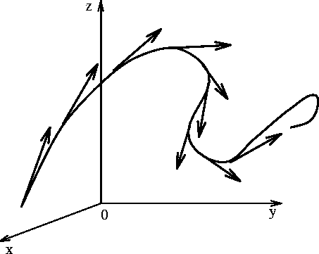
CurvatureThe curvature, at a given point, of a space curve is defined as the rate of change of the unit tangent vector with respect to arc length.
In other words the CURVATURE at a point tells you how fast is the
curve turning at that point. See the picture below.
 |
The formal definition of curvature is:
TheoremConsider a vector function f, but first some useful definitions for later, |
> i:=vector([1,0,0]):j:=vector([0,1,0]):k:=vector([0,0,1]):
> len:= proc(u) sqrt(innerprod(evalm(u),evalm(u))); end;
len := proc(u) sqrt(innerprod(evalm(u),evalm(u))) end> f := t -> x(t)*i + y(t)*j + z(t)*k;
f := t -> x(t) i + y(t) j + z(t) k
| The unit tangent is T, |
> Df := diff(f(t),t); D2f := diff(Df,t);
                    /  d      \     /  d      \     /  d      \
              Df := |---- x(t)| i + |---- y(t)| j + |---- z(t)| k
                    \ dt      /     \ dt      /     \ dt      /

                   /   2      \     /   2      \     /   2      \
                   |  d       |     |  d       |     |  d       |
            D2f := |----- x(t)| i + |----- y(t)| j + |----- z(t)| k
                   |   2      |     |   2      |     |   2      |
                   \ dt       /     \ dt       /     \ dt       /
> T := Df/len(Df): DT := diff(T,t):
.. I spare you the output...
| The curvature is then: |
> K := len( DT ) / len( Df ):
... Again big output that we don't need to look at...
| We now show that the curvature K has the alternative expression, Rhs, where |
> Rhs := len( crossprod( Df, D2f ) ) / len( Df )^3:
> simplify(Rhs^2 - K^2);
0
|
So YES! K = Rhs for all values of "t" and for all vector functions "f". Q.E.D. As usual it would be convenient to pack the curvature formula into a maple proc. |
> curvature := proc(f,t) local Df, D2f, l,u,v;
> Df := diff(f(s),s);
> D2f := diff(Df,s);
> Df := subs(s=t,Df);
> D2f := subs(s=t,D2f);
> u := crossprod(Df,D2f);
> l := sqrt(innerprod(u,u));
> RETURN(l/sqrt(innerprod(Df,Df))^3);
> end;
curvature := proc(f,t)
             local Df,D2f,l,u,v;
                 Df := diff(f(s),s);
                 D2f := diff(Df,s);
                 Df := subs(s = t,Df);
                 D2f := subs(s = t,D2f);
                 u := crossprod(Df,D2f);
                 l := sqrt(innerprod(u,u));
                 RETURN(l/sqrt(innerprod(Df,Df))^3)
             end
| Let's test it, |
> assume(r > 0): curvature(t->r*cos(t)*i+r*sin(t)*j,Pi);
                                        1
                                      ----
                                       r~
|
If you don't "assume" that r > 0 maple is not able to simplify this
much. So it works! Notice that this notion of curvature also agrees with
our intuitive idea of "curvature". As it is shown above, the curvature
of a circle of radius "r" is 1/r and the curvature is smaller the larger
the radius of the circle. The following picture shows how the "kissing" circle changes around the parabola y=x^2.
Exercise The DNA molecule has the shape of a double helix. The radius of each helix is about 10 angstroms (1 angstrom = 10^(-8) cm). Each helix rises about 34 angstroms during each complete turn and there are about 2.9 x 10^(8) complete turns. Estimate the length of each helix. |