| The prototypical example of a function of several variables is the Temperature at each point in a closed room. Each point in the room can be labeled with its three coordinates in a given coordinated system with basis elements i,j,k. Here are some examples of functions of several variables defined in maple: |
> T := (x,y,z) -> x^2+y^2+3*z^2;
                                          2    2      2
                         T := (x,y,z) -> x  + y  + 3 z
| This could represent a temperature field in a room. For example the temperature at (0,1,-1) = j-k is |
> T(0,1,-1);
4
| The volume V of a circular cylinder of radius r and hight h is also a function of several variables, but in this case of only 2. |
> V := (r,h) -> Pi*r^2*h;
                                               2
                             V := (r,h) -> Pi r  h
| As in the case of a vector function we can go back from an expression to the corresponding function by "unapply"-ing. For example: |
> g := unapply(sqrt(9-x^2-y^2),x,y);
                                             2    2 1/2
                         g := (x,y) -> (9 - x  - y )
| and we can now evaluate at different (x,y)'s with: |
> z1 := g(2,1); z2 := g(-1,Pi);
                                          1/2
                                   z1 := 4

                                            2 1/2
                               z2 := (8 - Pi )
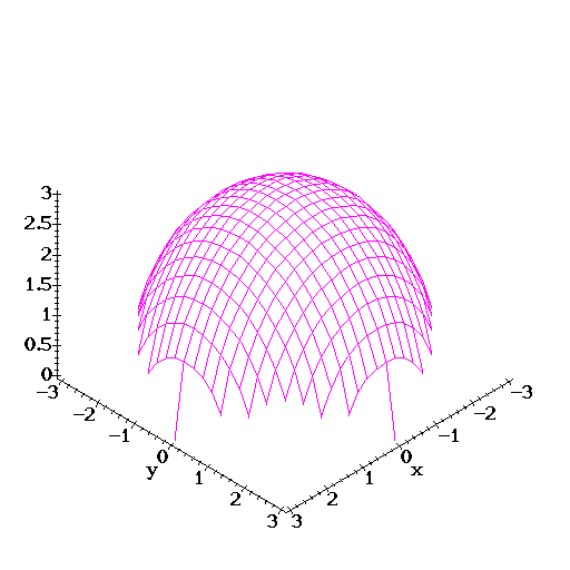
| Functions of two variables can be visualized as surfaces in 3D. For example |
> z := g(x,y);
                                        2    2 1/2
                             z := (9 - x  - y )
| can be seen as providing a rule for attaching a stick of length z to each point (x,y) in the circle of radius 3 centered at 0 on the xy-plane. We can look at it with: |
> plot3d(z,x=-3..3,y=-3..3,axes=framed,color=green);
Level CurvesThe level curves of a function of two variables are the curves where the function takes a constant value. The level curves have equations: |
> z := x*exp(-x^2-y^2);
                                           2    2
                             z := x exp(- x  - y )