• This lecture will be given by Prof. Zehnder of TAM, the other lecure, at 12:20 will be given by Prof. Terrell of the Math Department in Upson B17, and will not be placed on the Web.
• HW will be due at Monday lectures, starting 9/4.
• Computing HW details are posted on the web along with all other course information.

1. Vector Calculus.
   i.e. Line Integrals, Surface Integrals, Volume Integrals.
2. 1st and 2nd Order Ordinary Differential Equations.
3. Systems of 1st Order Differential Equations.
4. Fourier Series and Partial Differential Equations.

Some Examples

Systems of 1st Order Differential Equations

Imagine an island populated exclusively with rabbits and foxes
Let R(t), a function of time, be a continuous representation of the rabbit population
Let F(t), also a function of time, represent the fox population.

Given four constants of proportionality a,b,c,&d, we can create a model of how the populations change.
The Rabbit population will increase proportionally to the number of Rabbits already on the island, the more Rabbits, the more reproduction.
The Rabbit population will also decrease proportionally to the number of encounters Rabbits have with Foxes, which we can represent by the product of the number of Foxes and rabbits, R*F.
So, the rate of change of the Rabbits is dR/dt = aR - bRF
Similarly, the Fox population will decrease prportionally to the number of Foxes - the more Foxes the less rabbits (i.e. food) per Fox.
The Fox population will increase proportionally to the number of encounters of Foxes with Rabbits, represented again by R*F
The rate of change of the Foxes is then dF/dt = -cF + dRF

This is a system of 1st order differential equations, which can be analyzed numerically using techniques we'll learn later in the course. The resulting solution is an oscillatory one, i.e., like populations.

A Partial Differential equation is one that involves partial derivatives. An example would be the case of the temperature T, of a straight rod. The temperature is a function of both time and position. These dependancies are related in the heat equation:

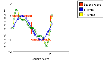
A graph shows how the series converges towards the square wave.

Line Integrals

A line integral is summing up (Integrating) a scalar quantity along a given line or curve.

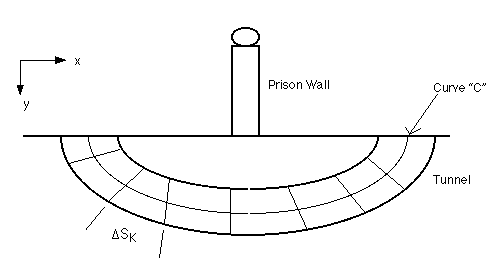
Imagine an inmate attempting to escape from prison. He has a tunnel plan all made out, but he'd like to know how much mass of dirt he's going to have to remove.

Suppose the density of the dirt is a function of depth - D(y).
The cross-sectional area of the tunnel is A.

To find out how much mass of dirt he has, the prisoner breaks up the tunnel plan into small sections. By approximating D in each section to be the average value for the section, he can add up the pieces.

1. Parametrize the path C - i.e. C consists of the points (x,y,z) where:
   x=x(t)
   y=y(t)
   z=z(t), a<=t<=b
   Or as a vector: r(t) = x(t)i + y(t)j + z(t)k

   An Example for a circular path:
   
   x(t) = R cos t
   y(t) = R sin t
   0<=t<=2*

   Define a "velocity" vector for a path as:
   v = dr/dt = dx/dt i + dy/dt j + dz/dt k.

   Now, back to the standard line integral form:
   

2. Along the path C defined, f(x,y,z) = f( x(t), y(t), z(t) ), making f a function only of t.

   If we take a small segment of the path we can see that, being nearly linear, it's differential length, ds, is equal to the speed, ||v||, times the differential time in traversing that length, dt. That is, ds = ||v|| dt

   
   So, the integral is now: