|
To find local max and min points of real valued functions of a single real variable you usually have to locate the points where the derivative
is zero. You probably learned in your first course on Calculus
that when the derivative is zero there is a good chance that you
are at the top of a hill or at the bottom of a valley but it is also
possible that the function is just changing concavity at that point
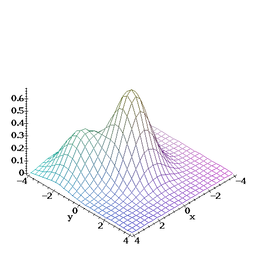
(remember the inflection points?). When dealing with a real valued function of two (or more) variables we can still talk about local max and mins and we shall find that the results in multivariate calculus will resemble the situation in Calc I although, in several dimensions there is more to worry about. Definition:A function of two variables has a local maximum at (a,b) if f(x,y) is less or equal than f(a,b) for all points (x,y) in some disk with center (a,b). On the other hand if f(x,y) is grater or equal than f(a,b) on such a disk then we say that f(a,b) is a local minimum value.Here is an example |
> f := (x,y) -> 2*exp(-(x^2+y^2)/2)/3 + exp(-((x-2)^2+(y+2)^2)/2)/3:
> plot3d(f(x,y),x=-4..4,y=-4..4,axes=frame);

| as you can see from the picture (can you see it?) this function has two local maximus at around (0,0) and at around (2,-2). The over all maximum of the function is at around (0,0). The over all max of a function is known as the global maximum. In this case: |
> Globalmax := f(0,0); localmax := f(2,-2);
                         Globalmax := 2/3 + 1/3 exp(-4)

                         localmax := 2/3 exp(-4) + 1/3
| or approximately |
> evalf(Globalmax), evalf(localmax);
.6727718797, .3455437592
| One way to find the location of the local extrema is to find where on the surface the tangent plane becomes parallel to the xy plane. Since the slopes of the tangent plane, along the x and y axis, are given by the partial derivatives of f w.r.t. x and y then we only need to find where these derivatives are BOTH zero. Unfortunately (see the example below) this technique sometimes fails to locate the local extrema. If the graph of the function is like the picture above, then there is no problem, and it is easy to find (with maple) the points where the partials are both zero. Just do: |
> fsolve({diff(f(x,y),x),diff(f(x,y),y)},{x,y});
{y = -1.893974104, x = 1.893974104}
| Maple needs to solve a system of two NON LINEAR equations in the unknowns x and y and this is sometimes tooooo difficult even for mighty maple to do! That's why above I only went for the approximate solution with "fsolve". Besides, we only got one of the two solutions. It is possible to help maple in its quest for the max by giving ranges for x and y like, |
> fsolve({diff(f(x,y),x),diff(f(x,y),y)},{x,y},{x=-0.5..0.5,y=-0.5..0.5});
{x = .01961636442, y = -.01961636442}
|
and this is a much more precise approximation to where the global max is achieved this is the peak showing around (0,0).
As I said above, knowing that the gradient is zero at some point does not mean that there is a local extremun there. There could be a saddle point i.e. a max in one direction but a min in the other. Here is an example: |
> g := (x,y) -> x^2 - y^2: gg := grad(g(x,y),[x,y]);
gg := [ 2 x, - 2 y ]
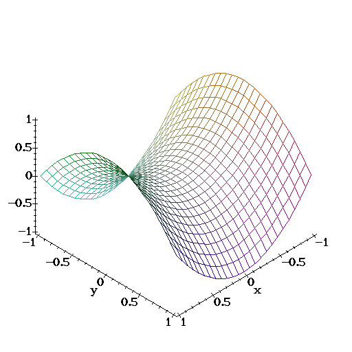
| Clearly gg=0 when x=y=0. But at (0,0) there is no local anything. g(x,0)=x^2 has a global min at x=0 but g(0,y)=-y^2 has a global max at y=0, a saddle! Here is the picture: |
> plot3d(g(x,y),x=-1..1,y=-1..1,axes=frame);
