| Recall the notion of a defined integral from Calc1. We denote by, |
> A = Int(f(x),x=a..b);
                                      b
                                      /
                                     |
                                A =  |  f(x) dx
                                     |
                                    /
                                    a
|
the integral of the function f over de interval [a,b]. The number "A"
is defined as a special limit and we say that the integral exists
and has "A" as its value, when this special limit exists. The idea
of integration is always the same. The integral of a function f
over some set D (included in the domain of definition of f) is
a limit and we say that the integral exists if this limit exists.
|
Riemann sums
The limit that defines an integral is of the same general form
for all integrals no matter if the function is
of one variable (as in calc1) or of several variables
(as here in calc3). This is what it takes:
Let's look at an example in two dimensions. Suppose that the function we want to integrate is: |
> f := (x,y) -> 3*x^2+(y-2)^2+2: vf := f(x,y): 'f(x,y)' = f(x,y);
                                      2          2
                         f(x, y) = 3 x  + (y - 2)  + 2
| and suppose further that we want to integrate this function over the rectangle R=[0,1]x[0,3]. This can be written as, |
> Int('f',A) = Int( Int('f(x,y)',x=0..1),y=0..3);
                                     3   1
                          /          /   /
                         |          |   |
                         |  f dA =  |   |  f(x, y) dx dy
                         |          |   |
                        /          /   /
                        R          0   0
| Maple can give you the answer right away with, |
> Int( Int('f(x,y)',x=0..1),y=0..3) = int( int(f(x,y),x=0..1),y=0..3);
                             3   1
                             /   /
                            |   |
                            |   |  f(x, y) dx dy = 12
                            |   |
                           /   /
                           0   0
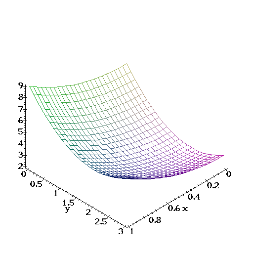
| but let's see that this value is really the result of taking the limit of sums as defined above. The graph of the function f over the rectangle R looks like this, |
> plot3d(vf,x=0..1,y=0..3,axes=frame);

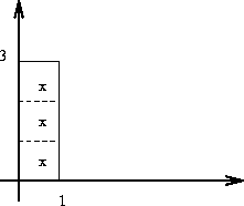
If we subdivide the rectangle of integration into three squares as
shown in the figure below,
 then the Riemann sum associated to this partition is: |
> Rsum1 := f(1/2,1/2)+f(1/2,3/2)+f(1/2,5/2);
Rsum1 := 11
| The following procedure computes the Riemann sum approximating the integral of a function f (which is an expression in x and y) over the rectangle R=[a,b]x[c,d]. Look at how to use this function after its definition below, |
> ApproxInt2d := proc(f,xexpress,yexpress,n,m)
> local a,b,c,d,dx,i,j,dy;
> a := op(1,op(2,xexpress));
> b := op(2,op(2,xexpress));
> c := op(1,op(2,yexpress));
> d := op(2,op(2,yexpress));
> dx := evalf((b-a)/n);
> dy := evalf((d-c)/m);
> sum(sum(subs(x = a+(i-.5)*dx,y = c+(j-.5)*dy,f),i = 1 .. n),j = 1 .. m)*dx*dy
> end:
| Let's try it first on the function f defined at the begining and see if we re-obtain Rsum1, |
> Rsum1_Now := ApproxInt2d(f(x,y),x=0..1,y=0..3,1,3);
Rsum1_Now := 11.
| Same thing!... so it looks ok. If we inprove the approximation by using now 6 rectangles (2 along x and 3 along y) we get: |
> Rsum2 := ApproxInt2d(f(x,y),x=0..1,y=0..3,2,3);
Rsum2 := 11.56250000
| and if we try to be cool and do: |
> RS := proc(m,n) ApproxInt2d(f(x,y),x=0..1,y=0..3,m,n) end:
| we can then look at how the sequence converges to its limit... |
> RS(1,3), RS(2,3), RS(3,4), RS(10,10), RS(100,100);
11., 11.56250000, 11.77604167, 11.97000000, 11.99970000
|
and to 12 it seems to go.
|
Iterated Integrals
|
Let us now use the RS proc above to demonstrate the fact that
the double integral of f(x,y) over the rectangle R=[a,b]x[c,d]
can be computed by integrating first with respect to y
(taking x as if it were a constant.. like in partial derivatives remember?)
and then integrate w.r.t. x the function of x that is obtained. In
this way the computation of a double integral is reduced to computing
two one dimensional (just as in calc1) integrals one after the other.
It is not difficult to see why the above method works. It is nothing but a computation of the Riemann sum, that is used to define the double integral, with the terms ordered in a different way. Look at the sequence of approximations that we generated above: 11, 11.56, 11.78,... etc. These numbers are the result of adding: 1*3=3, 2*3=6, 12, 100, and 10000 terms respectively. We are free to add the terms in each sum in any order we want, and as long as we add all of them the result will be the same. For example the 6 terms of the sum that produced 11.56 can be re-ordered as two terms each of them containing 3 numbers to be added. In other words, we fix one value for x and we add over all the values for y with that x fixed. Then we change the x to the next value and we again add over all the y's etc. Let's see what we get when x=1/2 and we increase the number of y's to add over: |
> RS(1,3), RS(1,30), RS(1,60), RS(1,200), RS(1,2000);
11., 11.24750000, 11.24937500, 11.24994375, 11.24999944
|
this seems to be going to 11.25 Notice that these numbers are approaching the limit that defines the integral, |
> Int('f(1/2,y)',y=0..3) = Int(f(1/2,y),y=0..3);
                     3                  3
                     /                  /
                    |                  |                2
                    |  f(1/2, y) dy =  |  11/4 + (y - 2)  dy
                    |                  |
                   /                  /
                   0                  0
| which in fact simplifies to: |
> Int(f(1/2,y),y=0..3) = int(f(1/2,y),y=0..3);
                           3
                           /
                          |                2
                          |  11/4 + (y - 2)  dy = 45/4
                          |
                         /
                         0
> evalf(45/4);
11.25000000
| if instead of fixing x=1/2 we let it be at a general x and we increase (as we did above when x was fixed at 1/2) the number of subdivisions on the y axis we obtain, |
> Int(f(x,y),y=0..3) = int(f(x,y),y=0..3);
                       3
                       /
                      |     2          2             2
                      |  3 x  + (y - 2)  + 2 dy = 9 x  + 9
                      |
                     /
                     0
| Notice that when x=1/2 we recover 45/4. So this says that for each value of x the sums over the y's (keeping x fixed) will approach the rhs of the above expression. To obtain the double integral we now need to add over all the x's and this will approach the value of the integral, |
> Int(9*x^2+9,x=0..1) = int(9*x^2+9,x=0..1);
                                1
                                /
                               |     2
                               |  9 x  + 9 dx = 12
                               |
                              /
                              0
| and we have shown that in this example (in fact this is always the case), |
> #
                                           b      d
                   /   /                   /  /   /           \
                  |   |                   |  | 	 |             |
                  |   |  f(x, y) dA   =   |  |	 |  f(x, y) dy | dx
                  |   |                   |  |	 |             |
                 /   /                   /   |	/              |
                   R                     a    \	c             /