| A line is determined by a direction vector v and a position vector u. |
> with(linalg):
> v := vector(3); u := vector(3);
                             v := array(1 .. 3, [])

                             u := array(1 .. 3, [])
|
Yes, this is the way in which maple tells that v and u
are two arbitrary vectors in 3 dimensional space.
The equation of the line with direction v and passing through u is: |
> Line := { u + t*v};
Line := {u + t v}
|
This is the set of all the vectors of the form: "position vector + a scalar multiple of the direction vector". The scalar "t" is a parameter that can take any value from -infinity to infinity. The position vector of every point on the line can be written as a function of the parameter "t" as follows: |
> L := t -> u + t*v;
L := t -> u + t v
u
u + v
| To see the coordinates of L(t) in the standard basis, just evalm: |
> evalm(L(t));
[ u[1] + t v[1], u[2] + t v[2], u[3] + t v[3] ]
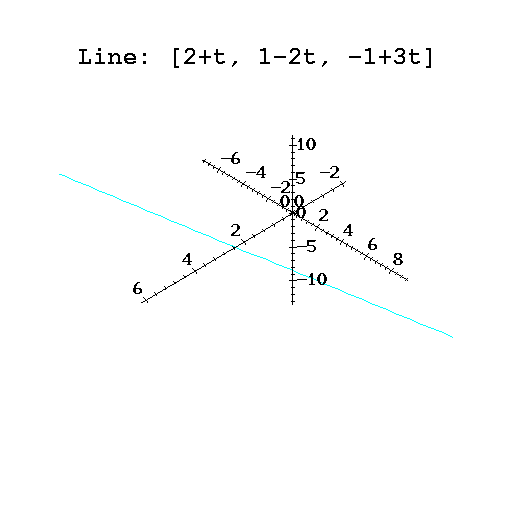
| The vector L(t) can be interpreted as the position at time "t" of a particle moving with constant velocity vector v that is found at position u at an innitial time 0. The following two commands will display a picture of the line with velocity vector [1,-2,,3] and position vector [2,1,-1]. |
> with(plots);
 [animate, animate3d, conformal, contourplot, cylinderplot, densityplot,

     display, display3d, fieldplot, fieldplot3d, gradplot, gradplot3d,

     implicitplot, implicitplot3d, loglogplot, logplot, matrixplot, odeplot,

     pointplot, polarplot, polygonplot, polygonplot3d, polyhedraplot, replot,

     setoptions, setoptions3d, spacecurve, sparsematrixplot, sphereplot,

     surfdata, textplot, textplot3d, tubeplot]
| Notice that the next command "spacecurve" was loaded with the "with" above. |
spacecurve([2+t, 1-2*t, -1+3*t], t=-4..4, axes=NORMAL, color=RED);
